5 Tests of Mean Differences for One- and Two-Sample Designs
(PSY206) Data Management and Analysis
A t-test compares an observed mean difference with the amount of variation expected if the null hypothesis were true. Its general form is
\[ t = \frac{\text{observed difference} - \text{difference under }H_0} {\text{estimated standard error of the difference}}. \]
Under the null hypothesis, the test statistic follows a t-distribution with an appropriate number of degrees of freedom. A large absolute value of \(t\) provides evidence against the null hypothesis.
The p-value is the probability, assuming \(H_0\) is true, of obtaining a test statistic at least as extreme as the one observed. It is not the probability that \(H_0\) is true.
1 Types of t-tests
There are three main types of t-test:
- One-sample t-test: compares the mean of one sample with a specified value, such as a population norm or chance level.
- Independent-samples t-test: compares the means of two separate and unrelated groups.
- Paired-samples t-test: compares two related measurements, such as measurements taken from the same participants before and after an intervention or observations from matched pairs.
1.1 Main assumptions
The assumptions differ slightly across the three tests.
| Assumption | One-sample | Independent samples | Paired samples |
|---|---|---|---|
| Quantitative outcome | Yes | Yes | Yes |
| Independent observations | Observations are independent | Observations are independent within and between groups | Pairs are independent of other pairs |
| Approximate normality | Outcome, especially for a small sample | Outcome within each group, especially for small groups | Pairwise differences, not necessarily the two raw variables |
| No influential extreme outliers | Yes | Yes | Yes, in the pairwise differences |
| Equal population variances | Not applicable | Required only for the pooled Student’s test, not Welch’s test | Not applicable |
The t-tests are often reasonably robust to moderate non-normality, particularly with larger samples and no severe outliers. For an independent-samples comparison, Welch’s t-test is generally safer when group variances or sample sizes differ.
When reporting a t-test, provide the relevant means, standard deviations, test statistic, degrees of freedom, p-value, confidence interval, and an effect size.
1.2 Two-sided and one-sided tests
A two-sided test asks whether a difference exists in either direction:
\[ H_0:\Delta=0 \qquad\text{versus}\qquad H_1:\Delta\ne0. \]
A one-sided test asks whether the difference is in a prespecified direction. For example,
\[ H_0:\Delta\le0 \qquad\text{versus}\qquad H_1:\Delta>0. \]
Use a one-sided test only when the direction was specified before examining the data and an effect in the opposite direction would not support the research hypothesis. Otherwise, use a two-sided test.
2 One-Sample t-Test
The one-sample t-test determines whether a population mean differs from a specified value, denoted by \(\mu_0\).
For a two-sided test,
\[ H_0:\mu=\mu_0 \qquad\text{versus}\qquad H_1:\mu\ne\mu_0. \]
The test statistic is
\[ t=\frac{\bar{x}-\mu_0}{s/\sqrt{n}}, \]
where \(\bar{x}\) is the sample mean, \(s\) is the sample standard deviation, and \(n\) is the sample size.
If \(H_0\) is true, then
\[ T\mid H_0\sim t_{n-1}. \]
Thus, the test has \(df=n-1\) degrees of freedom. The corresponding \(100(1-\alpha)\%\) confidence interval for the population mean is
\[ \bar{x}\pm t_{1-\alpha/2,n-1}\frac{s}{\sqrt{n}}. \]
2.1 Example Study: Assessing Memory
An enthusiastic teacher, who was also a psychology graduate, noticed that some children in her final-year primary class were frequently forgetful. For example, they forgot lunch boxes, sports kits, or homework.
She hypothesised that these children might have poorer long-term memory than the population norm. She administered a standardised long-term memory test with a published norm of 75% for children of that age. (Download score-data.xlsx)
A one-sample t-test was used to compare the class mean with 75%.
The hypotheses may be written as either:
- Two-sided: \(H_0:\mu=75\) versus \(H_1:\mu\ne75\); or
- Directional, if specified in advance: \(H_0:\mu\ge75\) versus \(H_1:\mu<75\).
2.1.1 Performing a One-Sample t-Test
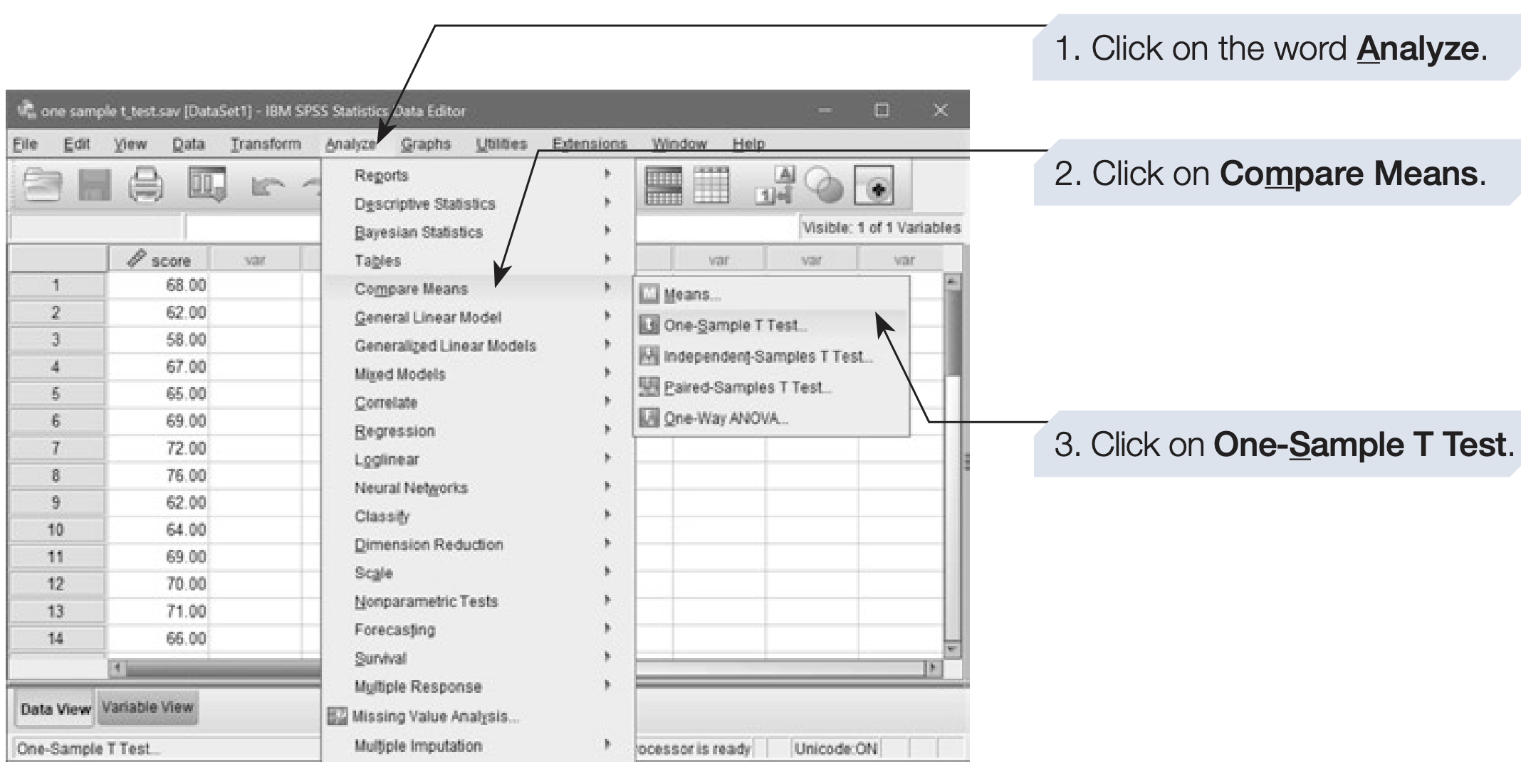
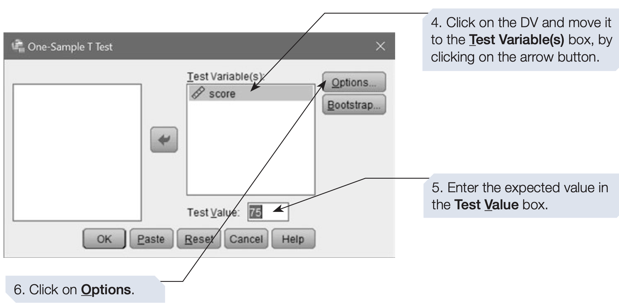
SPSS menu path:
Analyze → Compare Means → One-Sample T Test...SPSS syntax:
T-TEST
  /TESTVAL = 75
  /MISSING = ANALYSIS
  /VARIABLES = score
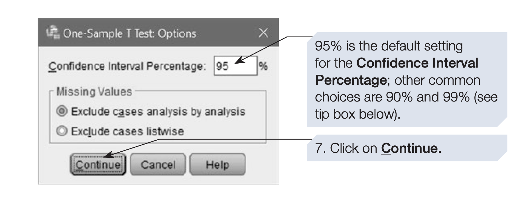
  /CRITERIA = CI(.95).
2.1.2 SPSS Output
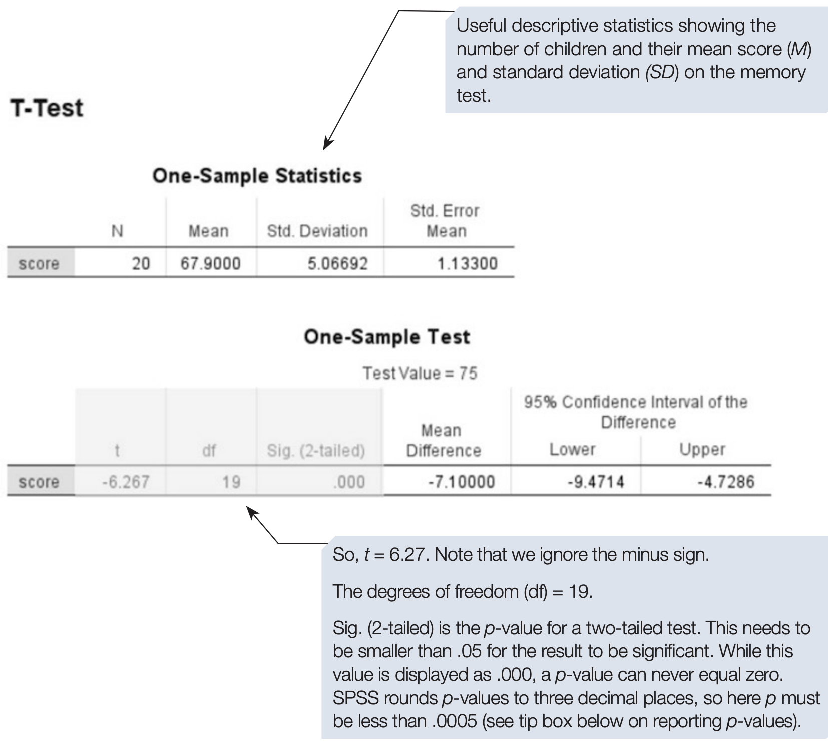
SPSS reports the sample statistics and then tests the difference
\[ \bar{x}-\mu_0=67.9-75=-7.1. \]
Using the rounded mean and standard deviation shown in the output,
\[ t=\frac{67.9-75}{5.07/\sqrt{20}}\approx-6.26. \]
SPSS calculates from the unrounded data and reports \(t=-6.27\). Under \(H_0\), \(T\sim t_{19}\). The negative sign shows that the sample mean is below the test value. Statistical significance is determined by the magnitude of \(t\) and its p-value, not by removing the sign.
2.1.3 Effect Size
For a one-sample t-test, Cohen’s \(d\) can be calculated as
\[ d=\frac{\bar{x}-\mu_0}{s}. \]
Here,
\[ d=\frac{67.9-75}{5.07}=-1.40. \]
The sign indicates direction; the absolute value indicates the size of the standardised difference.
2.1.4 Reporting the Results
Performance on the memory test was lower (\(M=67.9\%, SD=5.07\)) than the population norm of 75%. A one-sample t-test showed that the difference was statistically significant, \(t(19)=-6.27\), \(p<.001\), \(d=-1.40\).
- Report the t-statistic to two decimal places.
- Report the degrees of freedom inside parentheses: \(t(19)=-6.27\).
- Report exact p-values unless \(p<.001\).
- Do not include a leading zero for values that cannot exceed 1: write \(p=.045\), not \(p=0.045\).
- Report a confidence interval whenever possible.
3 Independent-Samples t-Test
The independent-samples t-test compares the population means of two separate groups. Examples include:
- males and females;
- a treatment group and a control group; and
- low-dose and high-dose drug groups.
Let \(\mu_1\) and \(\mu_2\) denote the two population means. For a two-sided comparison,
\[ H_0:\mu_1-\mu_2=0 \qquad\text{versus}\qquad H_1:\mu_1-\mu_2\ne0. \]
There are two versions of the independent-samples t-test.
3.1 Student’s t-Test: Equal Variances Assumed
When the two population variances can reasonably be treated as equal, the pooled variance is
\[ s_p^2= \frac{(n_1-1)s_1^2+(n_2-1)s_2^2} {n_1+n_2-2}. \]
The test statistic is
\[ t= \frac{(\bar{x}_1-\bar{x}_2)-\Delta_0} {s_p\sqrt{\frac{1}{n_1}+\frac{1}{n_2}}}, \]
where \(\Delta_0\) is the difference specified under \(H_0\), usually 0. Under \(H_0\),
\[ T\mid H_0\sim t_{n_1+n_2-2}. \]
Therefore,
\[ df=n_1+n_2-2. \]
3.2 Welch’s t-Test: Equal Variances Not Assumed
Welch’s test does not assume equal population variances. Its test statistic is
\[ t= \frac{(\bar{x}_1-\bar{x}_2)-\Delta_0} {\sqrt{\frac{s_1^2}{n_1}+\frac{s_2^2}{n_2}}}. \]
Under \(H_0\), the statistic is approximately t-distributed:
\[ T\mid H_0\approx t_{\nu}, \]
where the Welch-Satterthwaite degrees of freedom are
\[ \nu= \frac{\left(\frac{s_1^2}{n_1}+\frac{s_2^2}{n_2}\right)^2} {\frac{(s_1^2/n_1)^2}{n_1-1}+\frac{(s_2^2/n_2)^2}{n_2-1}}. \]
The value of \(\nu\) need not be a whole number.
SPSS reports both Equal variances assumed and Equal variances not assumed. The second row is Welch’s test.
Levene’s test evaluates \(H_0:\sigma_1^2=\sigma_2^2\). For two groups, its statistic is approximately \(F_{1,n_1+n_2-2}\) under \(H_0\). A small p-value indicates evidence of unequal variances. However, \(p>.05\) does not prove that the variances are equal. Examine group standard deviations, sample sizes, and outliers as well. When variances or sample sizes differ appreciably, use the Welch row.
3.3 Example Study: The Memory Experiment
In this example, we revisit the memory experiment introduced earlier (Chapter 2, download memory.sav).
The hypothesis was that participants who received mnemonic instructions would recall more words than those who did not. The groups contained different participants, so an independent-samples t-test was appropriate.
If the directional prediction was specified before examining the data, the hypotheses are
\[ H_0:\mu_{\text{Mnemonic}}-\mu_{\text{Non-mnemonic}}\le0 \]
and
\[ H_1:\mu_{\text{Mnemonic}}-\mu_{\text{Non-mnemonic}}>0. \]
3.3.1 Performing an Independent-Samples t-Test
SPSS menu path:
Analyze → Compare Means → Independent-Samples T Test...The grouping variable must identify the two groups, for example,
1 = Mnemonicand2 = Non-mnemonic.SPSS syntax:
T-TEST GROUPS = Condition(1 2)
  /VARIABLES = MemoryScore
  /MISSING = ANALYSIS
  /CRITERIA = CI(.95).
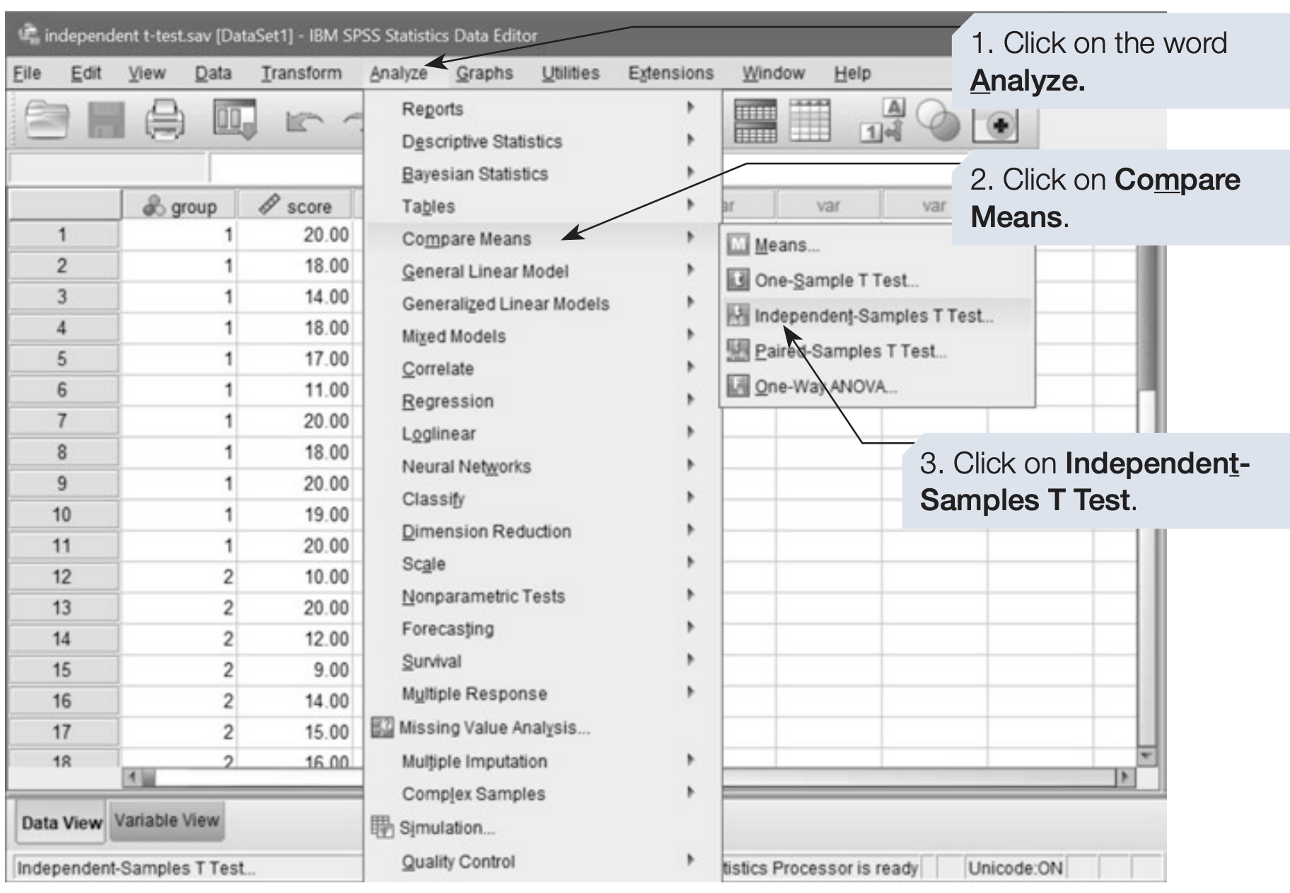
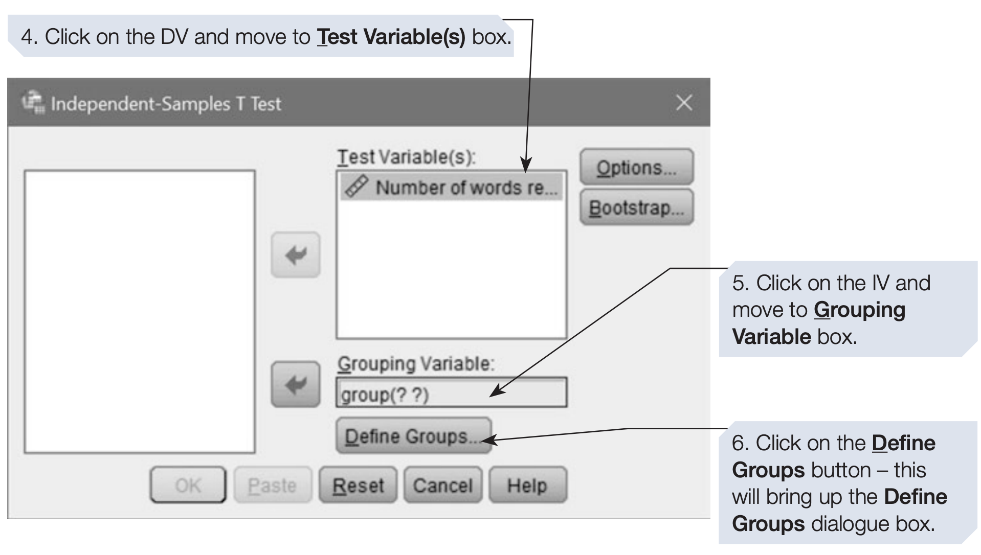
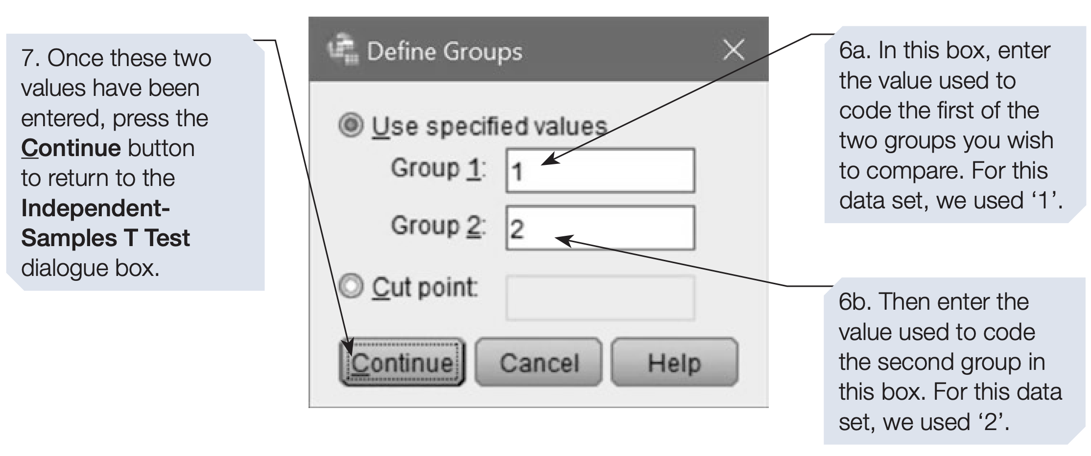
3.3.2 SPSS Output
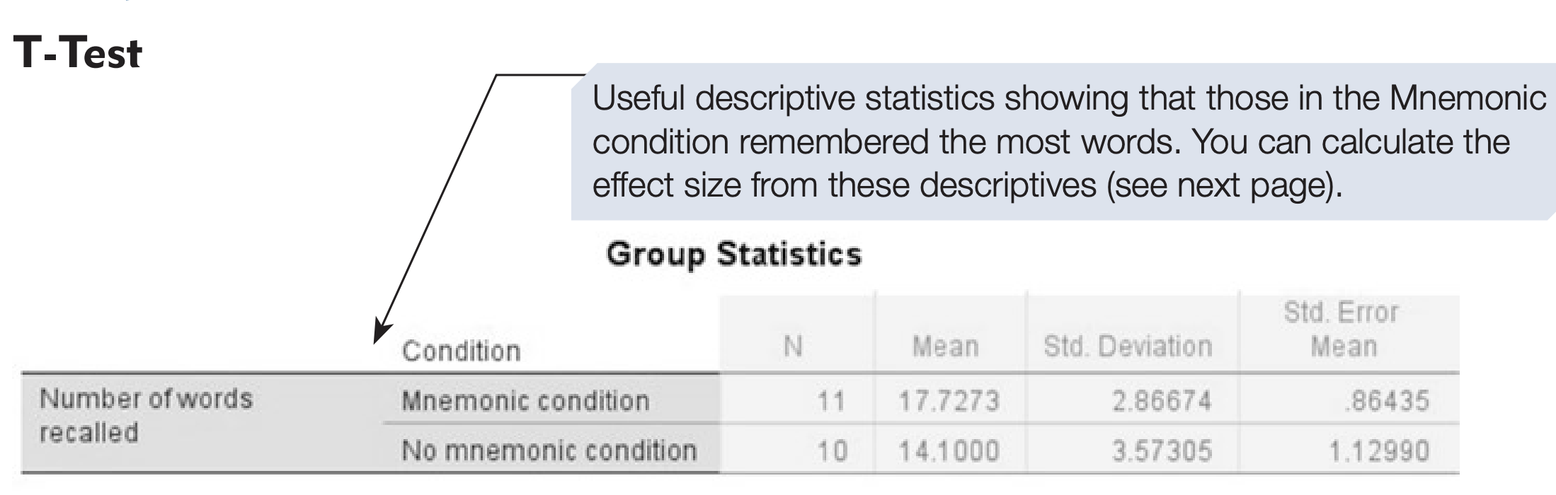
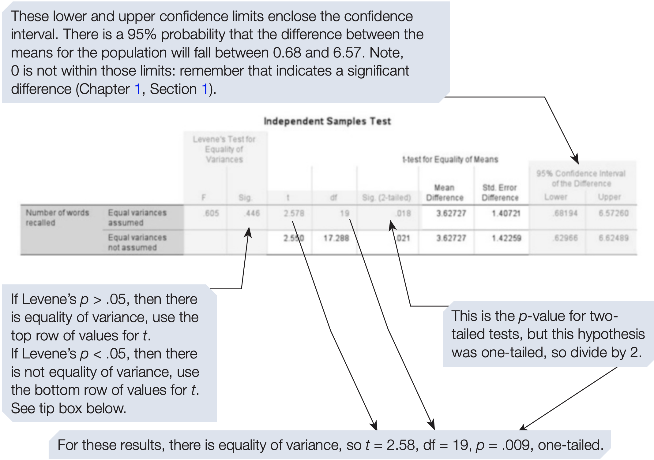
For the equal-variance analysis in this example, the pooled standard deviation is approximately \(s_p=3.22\). Therefore,
\[ t= \frac{17.73-14.10} {3.22\sqrt{\frac{1}{11}+\frac{1}{10}}} =2.58. \]
Under the null hypothesis, \(T\sim t_{19}\). The two-sided p-value is approximately .018. Because the observed difference is in the prespecified direction, the corresponding one-sided p-value is .009.
Use the one-sided p-value only when the directional hypothesis was set before analysing the data and the result is in that direction. Otherwise, report the two-sided p-value supplied by SPSS.
3.3.3 Effect Size
For the pooled independent-samples test, Cohen’s \(d\) is
\[ d=\frac{\bar{x}_1-\bar{x}_2}{s_p}, \]
where
\[ s_p= \sqrt{ \frac{(n_1-1)s_1^2+(n_2-1)s_2^2} {n_1+n_2-2} }. \]
For this study,
\[ d=\frac{17.73-14.10}{3.22}=1.13. \]
This means that the group means differed by approximately 1.13 pooled standard deviations. For small samples, Hedges’ \(g\) may be reported because it applies a small-sample correction to Cohen’s \(d\).
3.3.4 Reporting the Results
Participants in the Mnemonic condition (\(M=17.73\), \(SD=2.87\)) recalled more words than participants in the Non-mnemonic condition (\(M=14.10\), \(SD=3.58\)). The difference was statistically significant, \(t(19)=2.58\), \(p=.009\) (one-sided), 95% CI for the mean difference \([0.68, 6.58]\), \(d=1.13\).
If a directional test had not been specified in advance, the same result should be reported with the two-sided value, \(p=.018\).
3.4 Creating an Error Bar Graph
An error bar graph can display each group mean with its 95% confidence interval.
For the mnemonic memory study:
- Mnemonic: \(M=17.73\), 95% CI \([15.80, 19.65]\);
- Non-mnemonic: \(M=14.10\), 95% CI \([11.54, 16.66]\).
3.4.1 Creating the Graph in SPSS
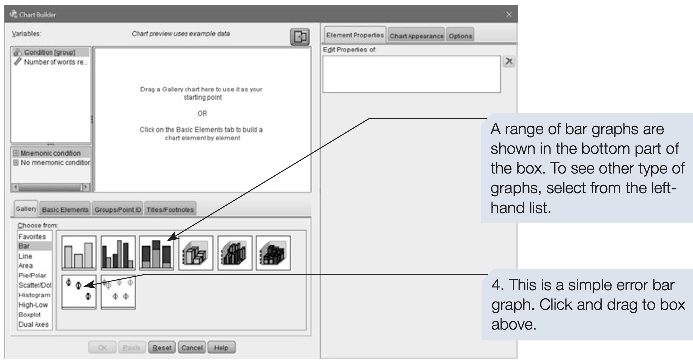
- Select Graphs → Chart Builder.
- Close the reminder about measurement levels if it appears.
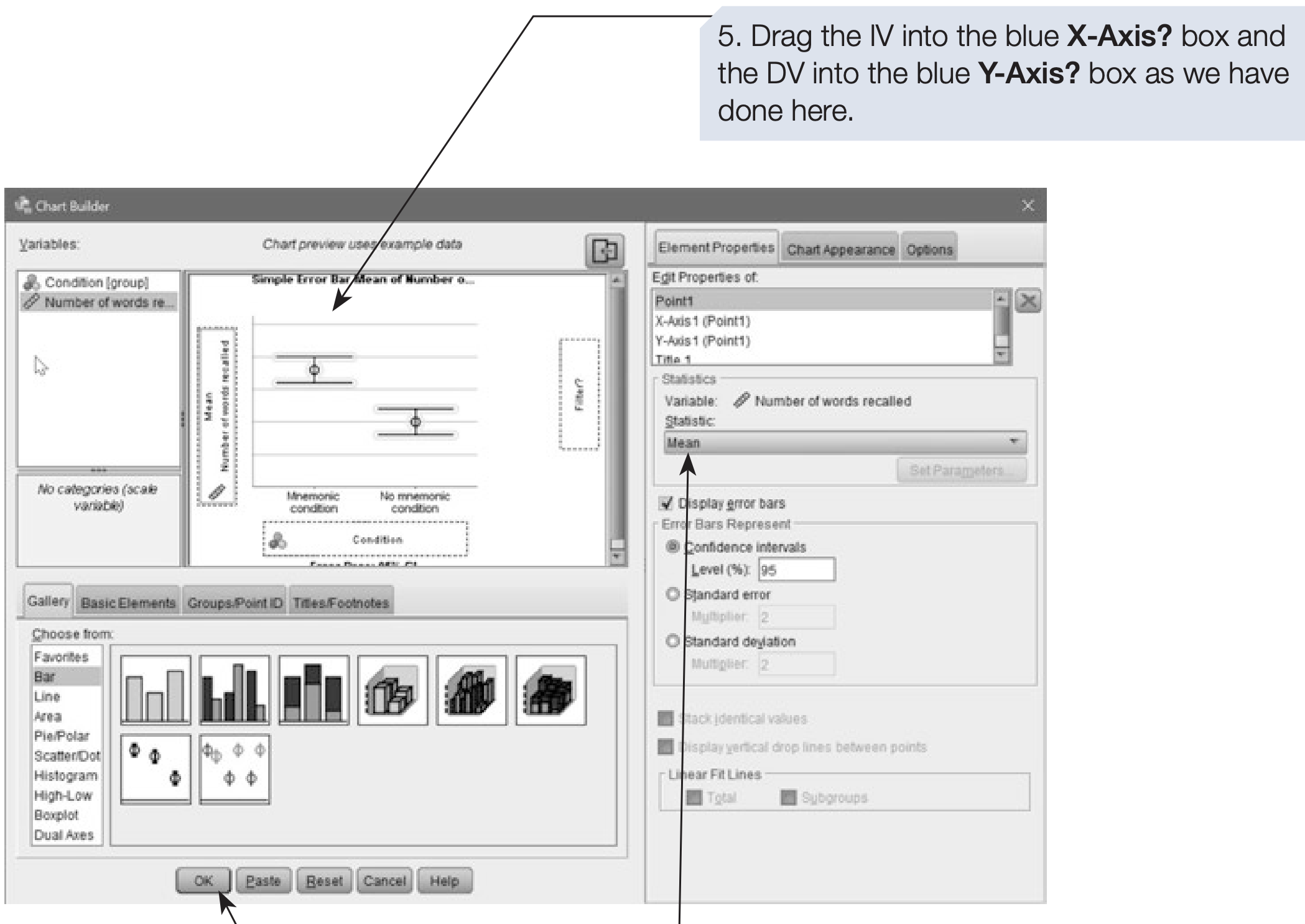
- Select an error bar graph and place the outcome on the y-axis and the group variable on the x-axis.
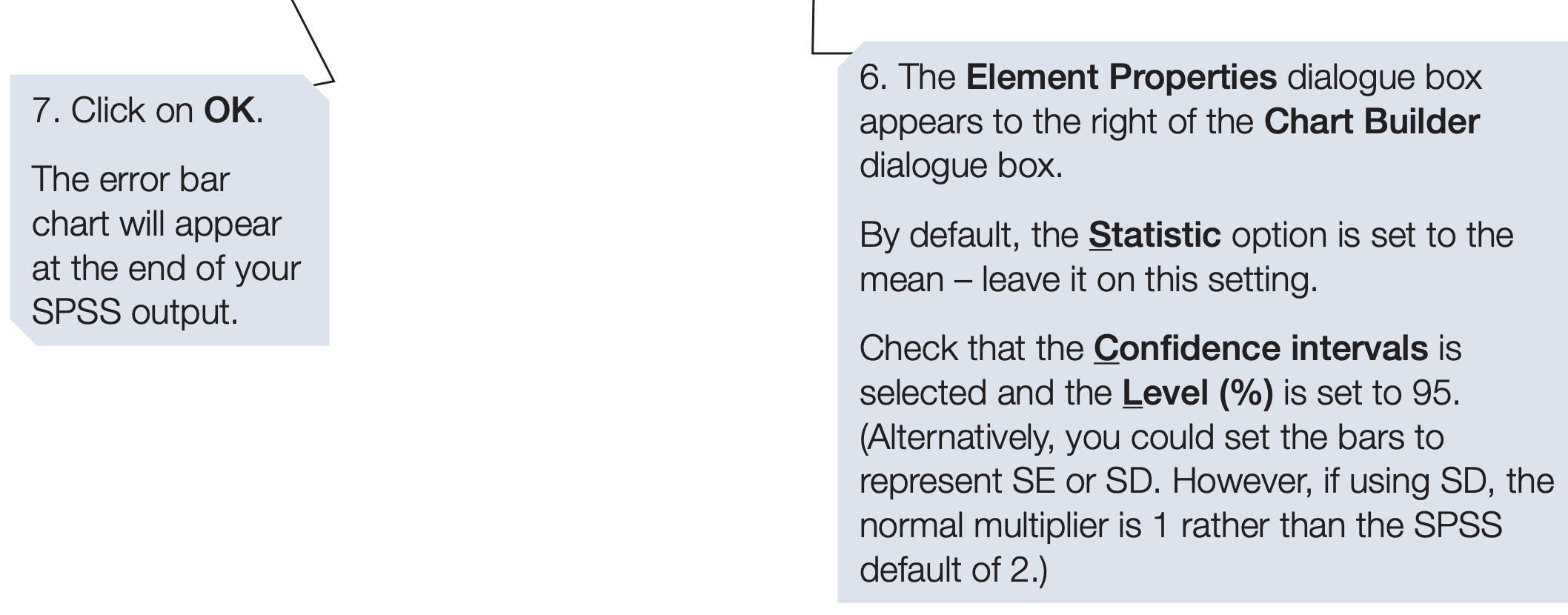
- In Element Properties, display the mean and 95% confidence interval.
3.4.2 SPSS Output
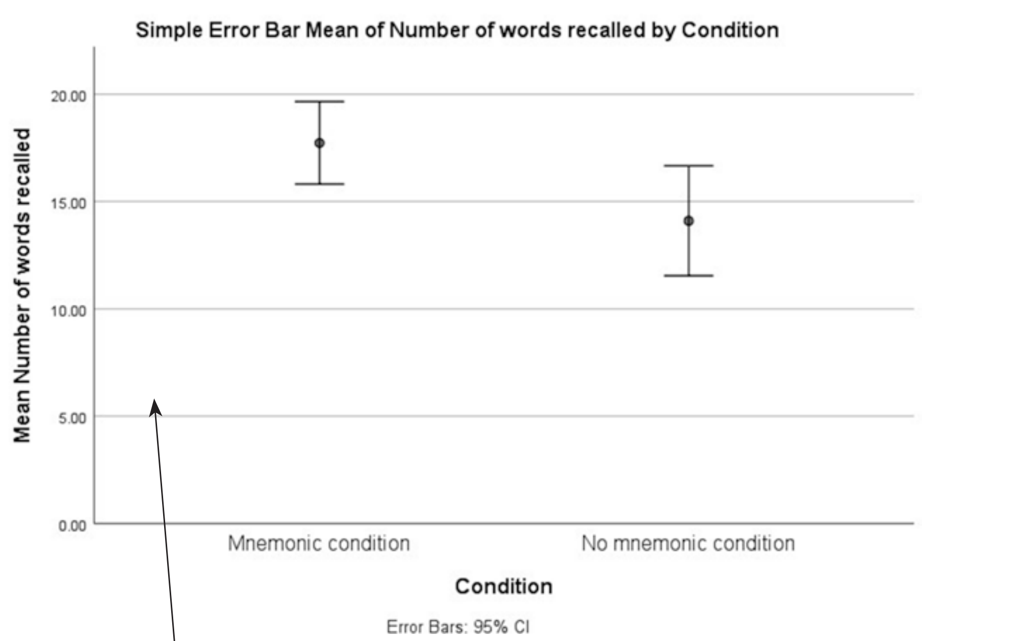
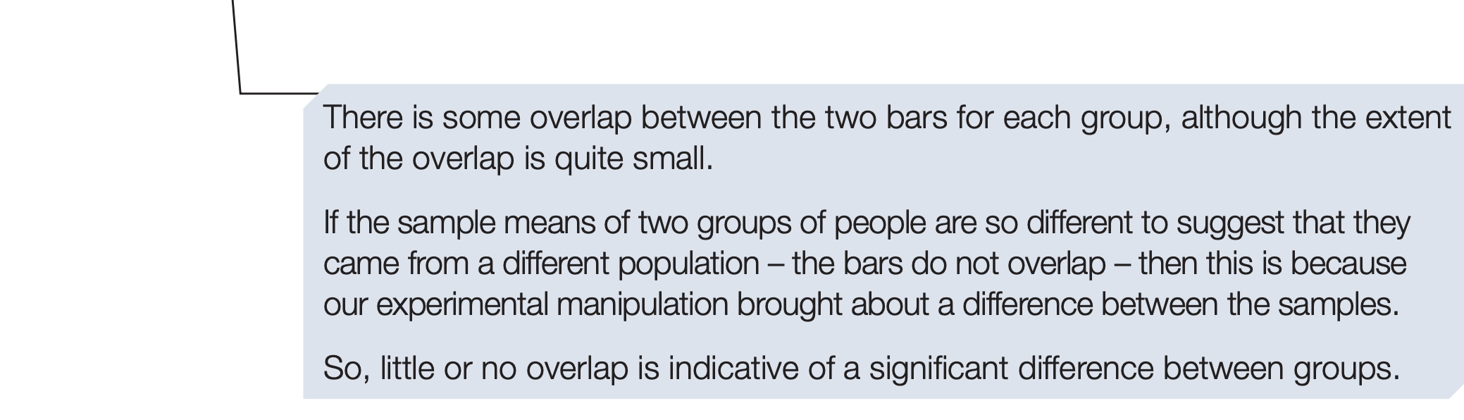
Do not decide statistical significance only by looking at whether the two group confidence intervals overlap. The independent-samples t-test uses the standard error of the difference between means, which is not the same as comparing two separate confidence intervals.