3 Exploring Data: Descriptive Statistics and Graphs
(PSY206) Data Management and Analysis
1 Descriptive Statistics
- Descriptive statistics are methods used to summarize and describe the main characteristics of a dataset using numerical measures, tables, and graphs.
- They help us:
- understand the distribution and characteristics of the data;
- identify unusual or potentially problematic observations;
- compare groups;
- communicate results clearly.
A few well-chosen descriptive measures and graphs can often communicate the main features of a large dataset effectively.
Common descriptive summaries include:
- Measures of central tendency
- Mean
- Median
- Mode
- Measures of variability (dispersion)
- Minimum and maximum
- Range
- Interquartile range (IQR)
- Variance
- Standard deviation
- Measures of position
- Percentiles
- Quartiles
Important: Descriptive statistics describe the observed data. They do not, by themselves, establish causal relationships or provide evidence for a statistical hypothesis.
In this chapter, we will learn how to obtain descriptive statistics and graphs using SPSS.
Most statistical procedures in SPSS can produce relevant descriptive information. However, SPSS also provides dedicated procedures for exploring data.
Two commonly used procedures are: 1. Descriptives, 2. Frequencies
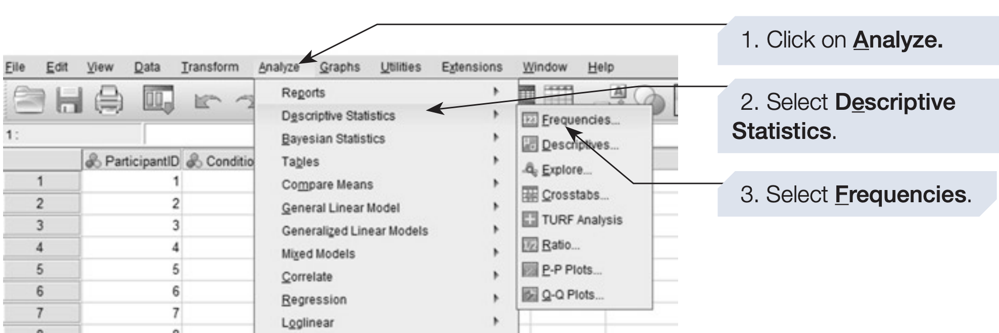
Both are available under: Analyze > Descriptive Statistics
2 The Descriptives Command
In this section, we will use the dataset from the Independent Groups Study of Memory, created in Chapter 2. (download memory.sav)
We will use the Descriptives command to obtain basic numerical summaries and examine how SPSS presents the results.
2.1 Steps to Access the Descriptives Command
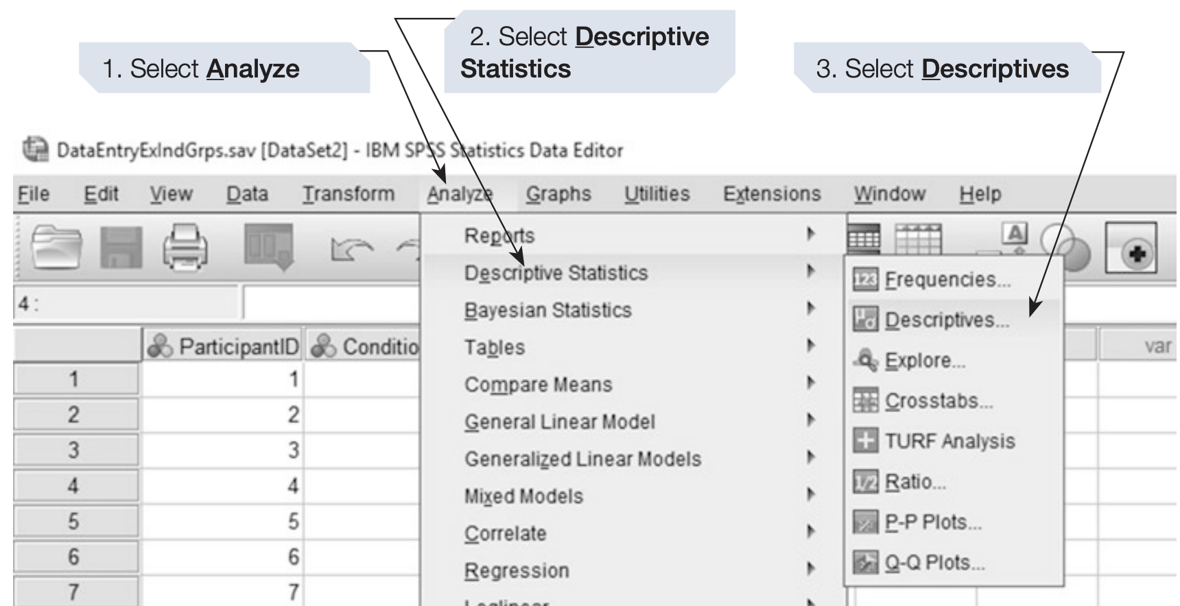
SPSS will display the Descriptives dialog box.
2.2 Understanding the Dialog Box
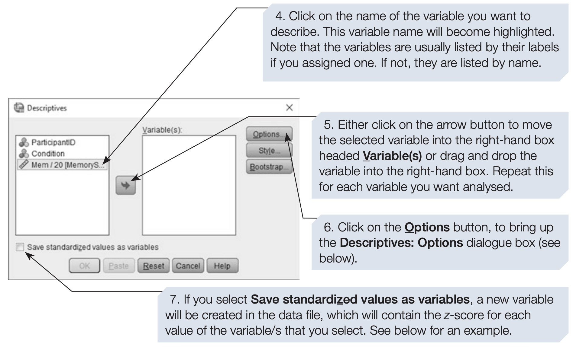
The dialog box follows a structure that is common to many SPSS procedures.
- The left panel lists the variables available in the dataset.
- The right panel lists the variables selected for analysis.
- Variables can be moved from the left panel to the right panel using the arrow button or by dragging and dropping.
Select MemoryScore and move it to the Variable(s) box.
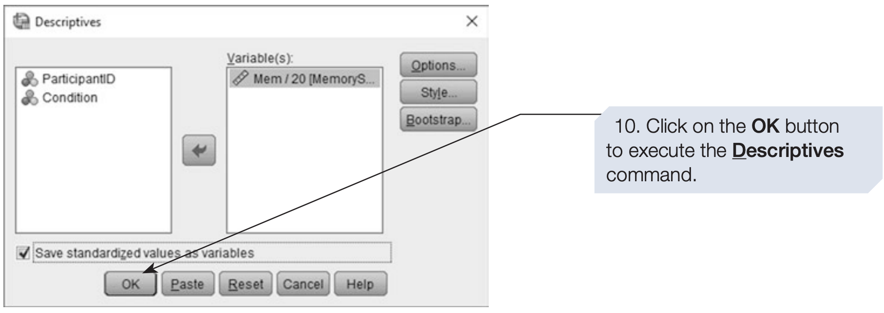
Click OK to execute the Descriptives command.
2.3 The SPSS Viewer Window
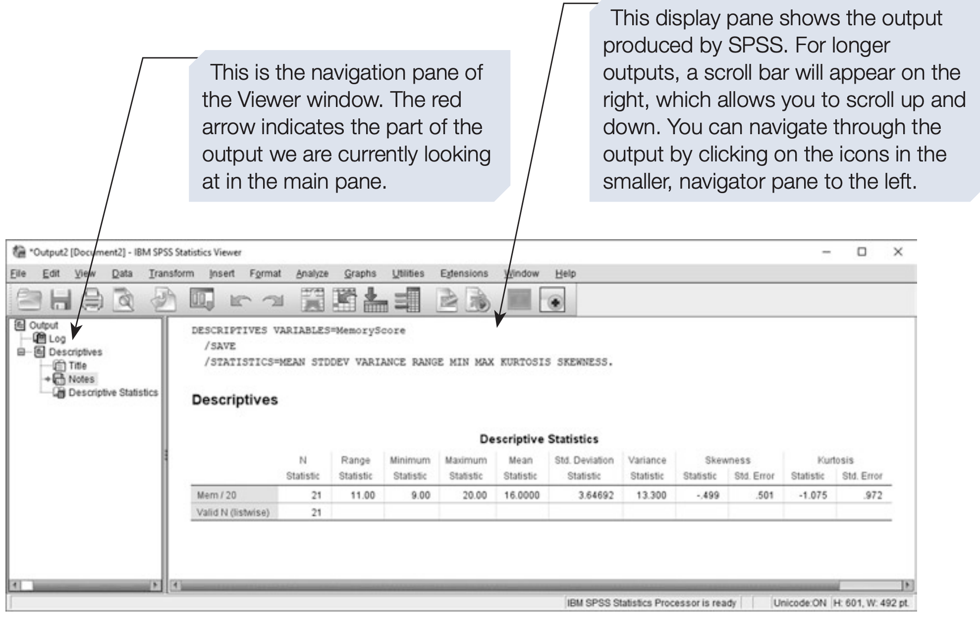
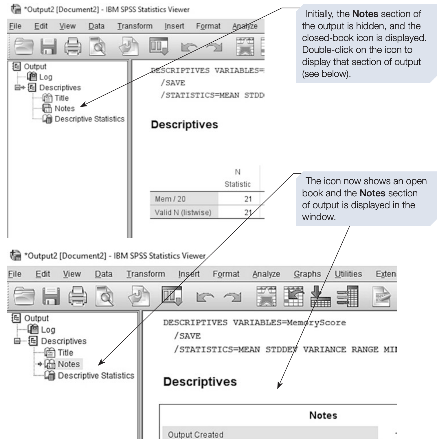
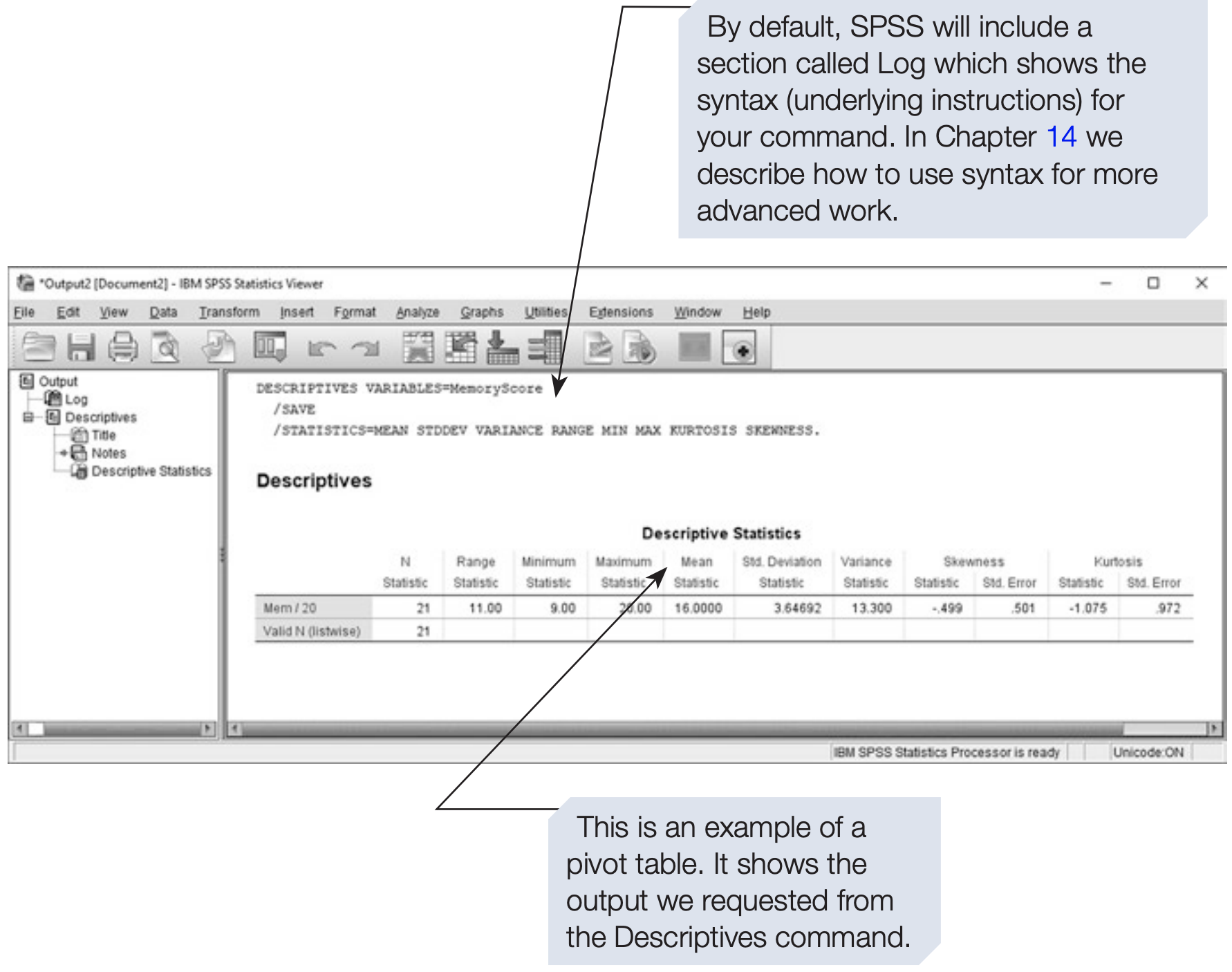
After running a procedure, SPSS displays the results in the Viewer window.
- If a Viewer window is already open, the new output is added to it.
- Otherwise, SPSS opens a new Viewer window.
- The output may contain tables, charts, and other results.
2.4 Managing the Output
You can:
- Copy output into other applications.
- Paste output into reports or presentations.
- Edit tables and charts.
- Export output to other file formats.
To remove output, select the relevant item in the Navigator pane and press Delete.
3 The Frequencies Command
The Frequencies command is particularly useful for exploring categorical and discrete variables.
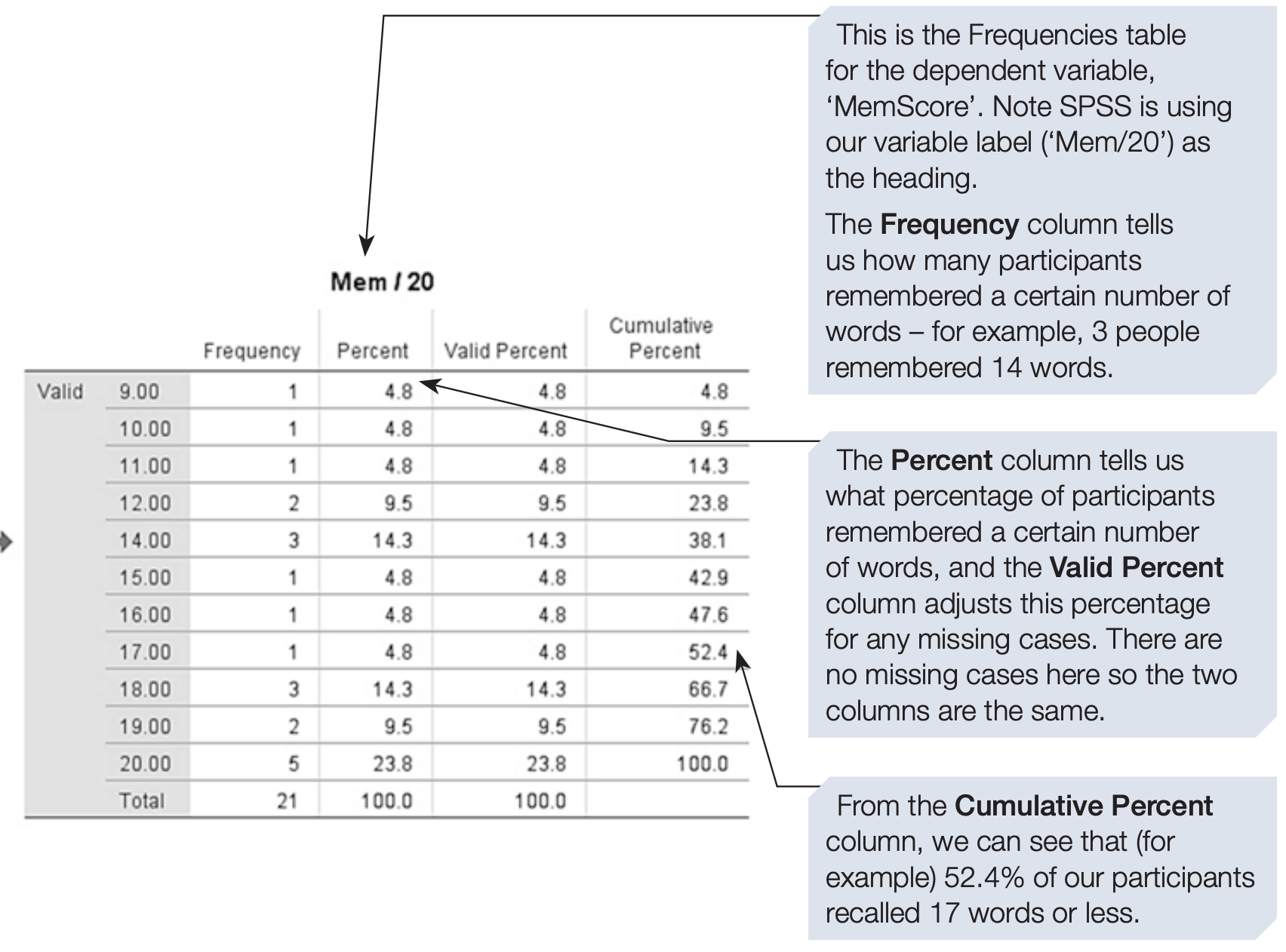
It produces a frequency table showing how often each value or category occurs.
For example, if Condition is coded as:
1 = Mnemonic
2 = Non-mnemonic
a frequency table can show the number and percentage of participants in each group.
3.1 Steps to Obtain Frequency Tables
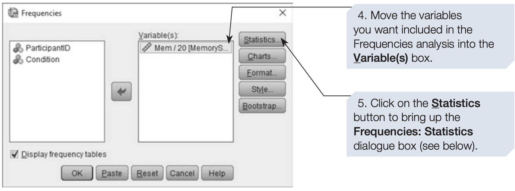
3.2 Selecting Variables
- Select one or more variables for the frequency analysis.
- Move them into the Variable(s) box using the arrow button or by dragging and dropping.
3.3 Output
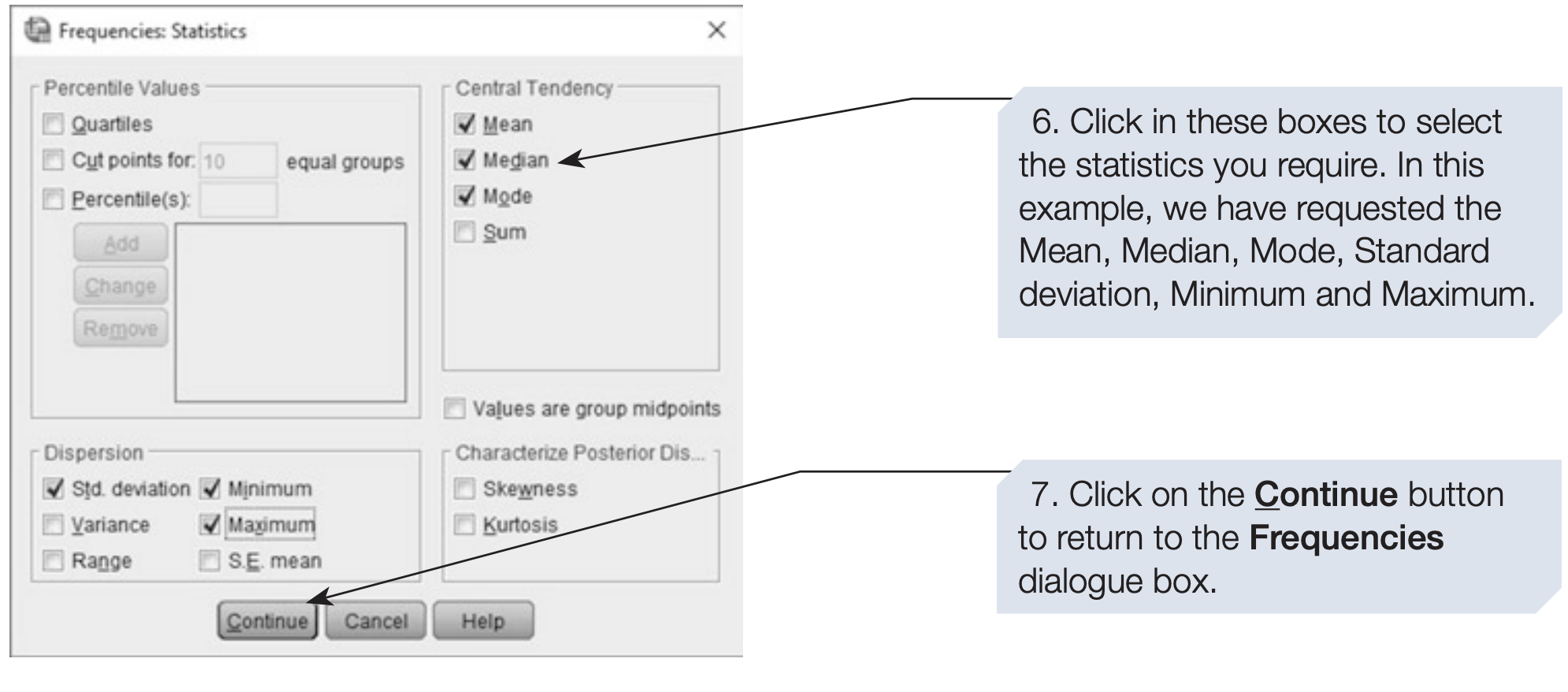
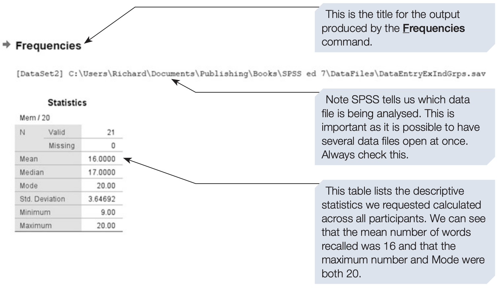
The output from the Frequencies command may include:
- A frequency table.
- Frequency counts.
- Percentages.
- Valid percentages.
- Cumulative percentages.
- Descriptive statistics.
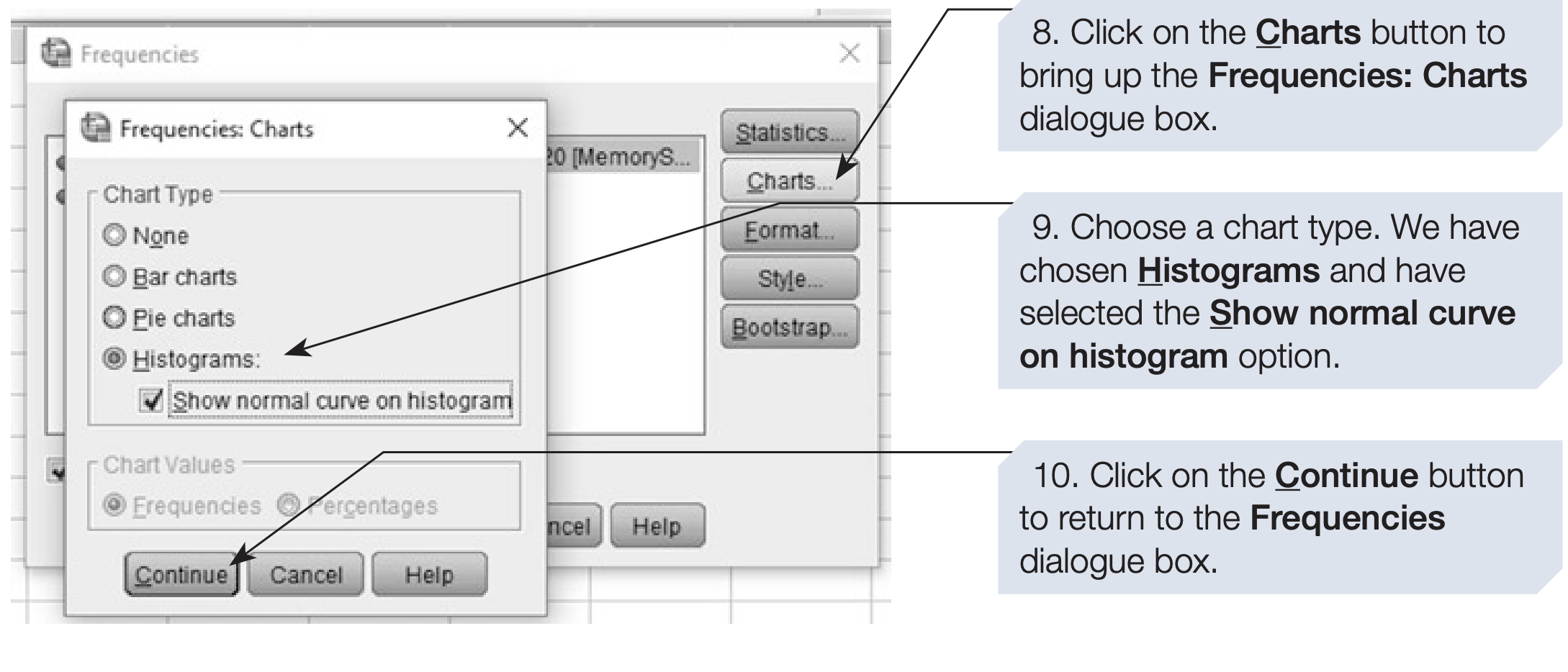
- Bar charts.
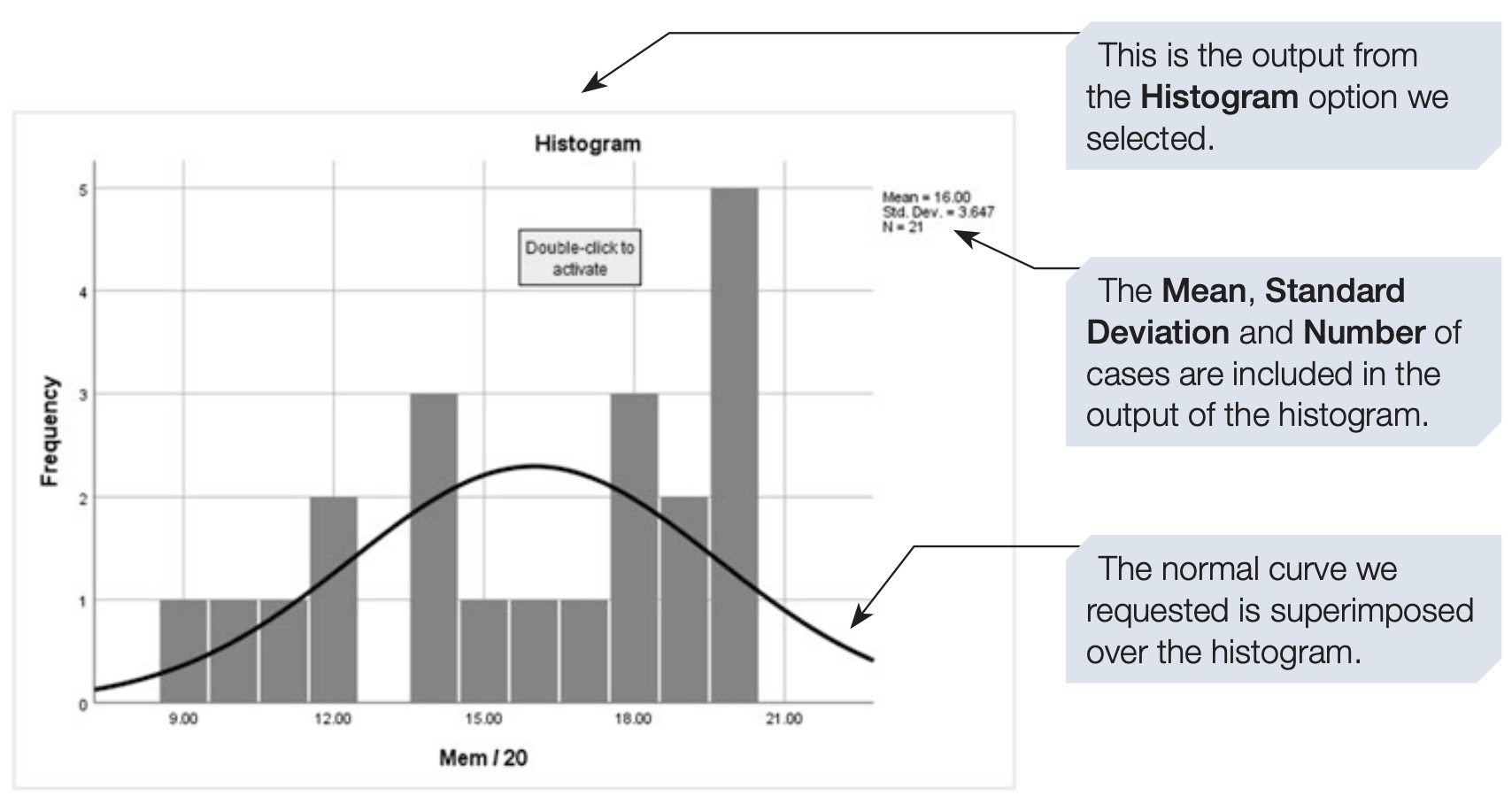
- Histograms.
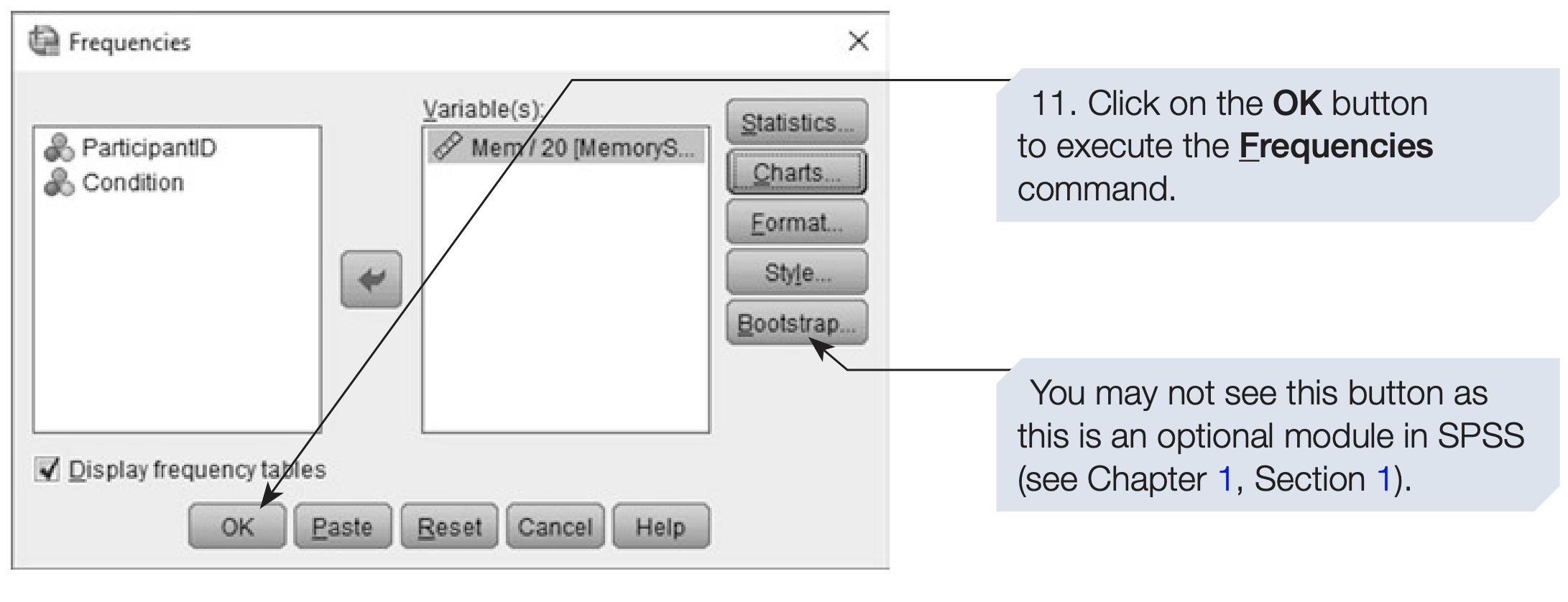
The exact output depends on the options selected.
4 Producing Graphs in SPSS
Numerical summaries are useful, but graphs can often reveal features of the data that are difficult to see from numbers alone.
Graphs can help us identify:
- The shape of a distribution.
- Differences between groups.
- Trends over time.
- Relationships between variables.
- Potential outliers.
- Unusual or unexpected observations.
SPSS provides several ways to create graphs.
Some statistical procedures, such as Frequencies, include graphing options. SPSS also provides dedicated graphing tools through the Graphs menu.
In this chapter, we will introduce several important graph types:
- Boxplots
- Histograms
- Bar charts
- Scatterplots
5 Boxplot
A boxplot, also called a box-and-whisker plot, provides a compact summary of the distribution of a quantitative variable.
A typical boxplot displays:
- Median: the line inside the box.
- First quartile (Q1): the lower edge of the box.
- Third quartile (Q3): the upper edge of the box.
- Interquartile range (IQR): the height of the box, where \(IQR =Q_3-Q_1.\)
- Whiskers: extend from the box to observations within the usual non-outlier range.
- Potential outliers: may be displayed separately from the whiskers.
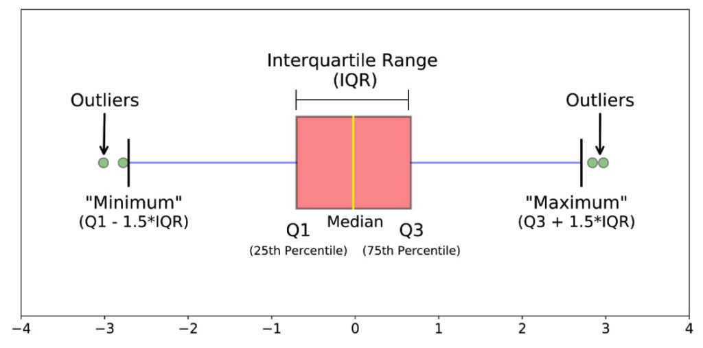
The exact rules SPSS uses to identify and display outliers should be checked in the specific graph.
5.1 When should we use a boxplot?
Boxplots are particularly useful when:
- The variable is quantitative.
- We want to examine the distribution of a variable.
- We want to compare distributions across groups.
- We want to identify possible outliers.
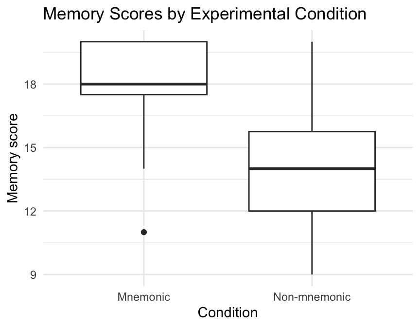
5.2 Example
Suppose we want to compare MemoryScore between two groups:
- Mnemonic instruction
- Non-mnemonic
A boxplot can display one box for each group.
If the median MemoryScore is higher in the mnemonic group, its boxplot will generally be positioned higher on the vertical axis.
The boxplot may also reveal whether one group has:
- greater variability;
- a different median;
- a different overall range;
- potential outliers.
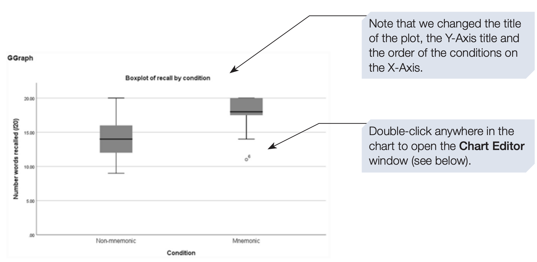
Interpretation: As the mnemonic group’s box is generally higher than the non-mnemonic group’s box, the mnemonic group tends to have higher memory scores.
6 Histogram
A histogram displays the distribution of a quantitative variable by dividing its values into intervals, called bins, and showing the frequency in each interval.
Unlike a bar chart, the bars in a histogram normally touch, because the intervals represent adjacent parts of a numerical scale.
A histogram can help us assess:
- Centre
- Spread
- Shape
- Skewness
- Possible outliers
- Possible multiple peaks
6.1 When should we use a histogram?
Histograms are appropriate for quantitative variables such as:
- Age
- Height
- Weight
- Income
- Test scores
- Memory scores
They are especially useful when we want to understand the shape of a distribution.
6.2 Example
Suppose MemoryScore ranges from 8 to 20. A histogram might show how many participants scored:
- 8–10
- 11–12
- 12–14
- 16–19
- 19-20
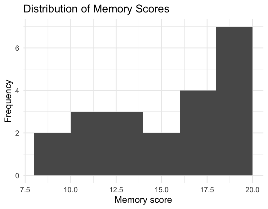
Interpretation: A histogram with most observations between 16 and 20 suggests that participants generally recalled a relatively large number of words.
7 Bar Chart
A bar chart displays frequencies, percentages, or other summary statistics for separate categories.
Bar charts are commonly used for:
- Nominal variables
- Ordinal variables
- Group comparisons
The height or length of a bar represents the value being displayed.
Because the categories are distinct, the bars are normally separated by gaps.
7.1 When should we use a bar chart?
Use a bar chart when the main variable on the horizontal axis is categorical.
Examples include:
- Sex
- Marital status
- Education level
- Treatment group
- Religion
- Employment status
7.2 Example 1: Frequency Bar Chart
Suppose Condition has two categories:
1 = Mnemonic
2 = Non-mnemonic
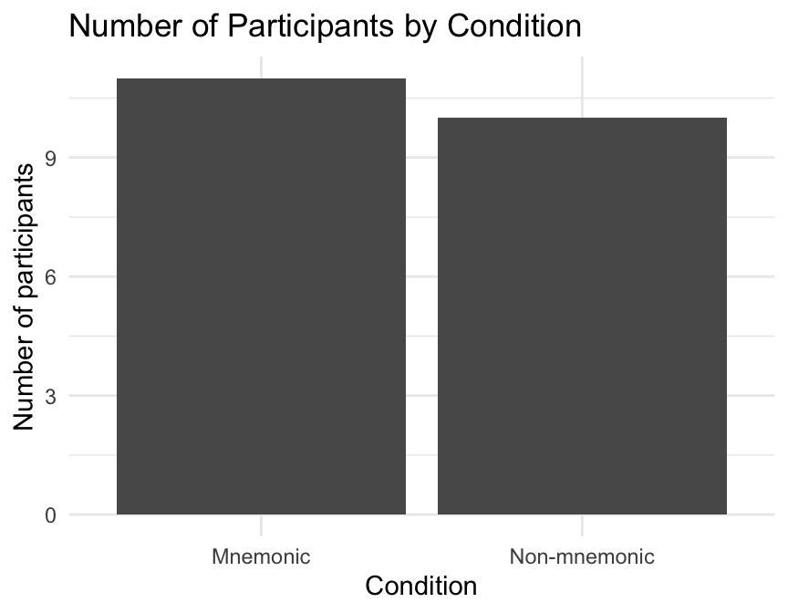
A bar chart can show the number of participants in each condition.
If there are 11 participants in the mnemonic group and 10 in the non-mnemonic group, the mnemonic bar will be slightly taller.
7.3 Example 2: Bar Chart of Means
Bar charts can also compare a summary statistic across groups.
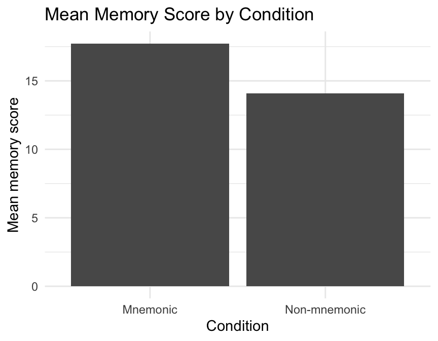
For example, we could display the mean MemoryScore for:
- Mnemonic group
- Non-mnemonic group
Each bar would represent the mean score of one group.
7.4 Histogram vs Bar Chart
This distinction is important:
| Histogram | Bar.Chart |
|---|---|
| Usually for quantitative variables | Usually for categorical variables |
| Values are grouped into numerical intervals | Each bar represents a category |
| Bars usually touch | Bars normally have gaps |
| Shows distribution | Shows comparison of categories |
8 Scatterplot
A scatterplot displays the relationship between two quantitative variables.
Each point represents one observation. For each observation:
- The x-coordinate represents the value of one variable.
- The y-coordinate represents the value of another variable.
8.1 When should we use a scatterplot?
Scatterplots are useful for examining:
- Direction of association — positive, negative, or no clear direction.
- Strength of association — how closely the points follow a pattern.
- Form of association — whether the relationship appears linear or non-linear.
- Clusters — whether observations form distinct groups.
- Potential outliers — observations that appear unusual compared with the overall pattern.
8.2 Example
Suppose we have data on individuals’ age and critical flicker fusion (CFF). CFF measures the speed at which your visual system can process a flickering light before it appears as a steady beam. (download age_cff_data.xlsx)
The dataset is stored in an Excel file containing two variables:
age— age of the individual.cff— critical flicker fusion value.
We can use a scatterplot to investigate whether CFF tends to change with age.
In the scatterplot:
- Age is placed on the x-axis.
- CFF is placed on the y-axis.
- Each point represents one individual.
A fitted linear trend (optional) can be added to help us see the overall direction of the relationship:
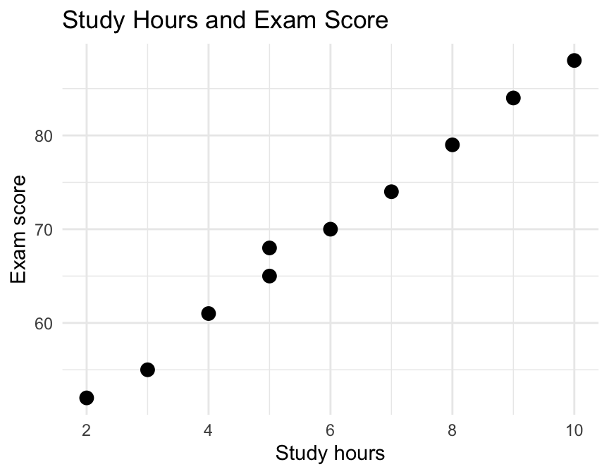
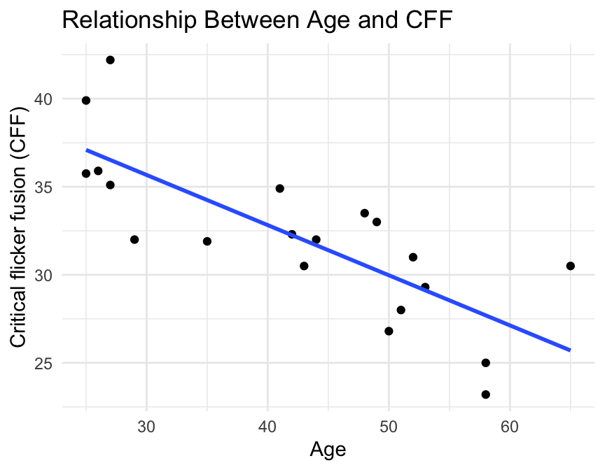
The points show the individual observations, while the line shows the estimated linear trend.
Interpretation: Examine the overall pattern of the points. If the points tend to decrease as age increases, this suggests a negative association between age and CFF. If they tend to increase, this suggests a positive association. If there is no clear pattern, there may be little or no obvious association. The scatterplot should be examined before drawing a conclusion about the relationship.
Important caution:
A scatterplot can show association, but association does not establish causation.
For example, even if age and CFF are negatively associated, the scatterplot alone cannot establish that increasing age causes CFF to decrease. Other factors may also be related to both variables.
9 The Chart Builder
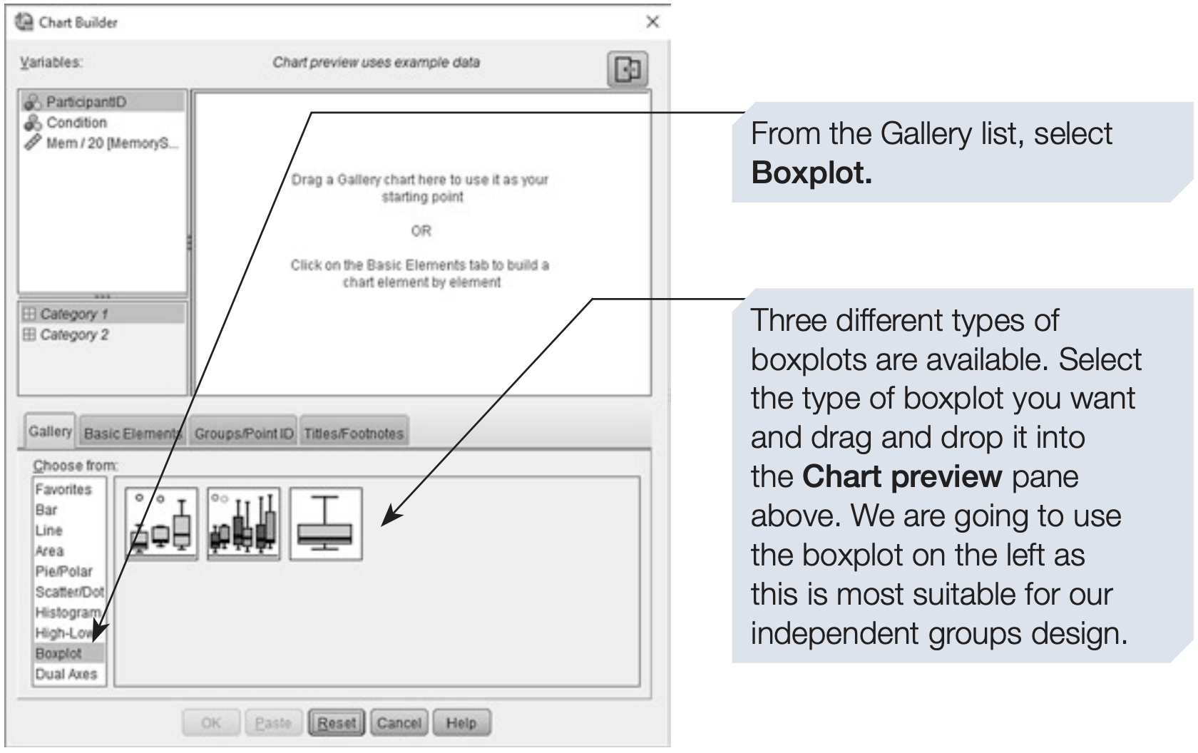
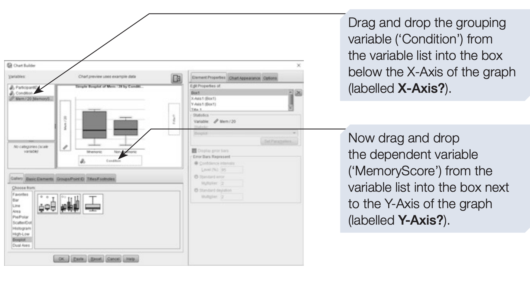
We will now demonstrate how to use the Chart Builder to produce a boxplot for the memory study dataset.
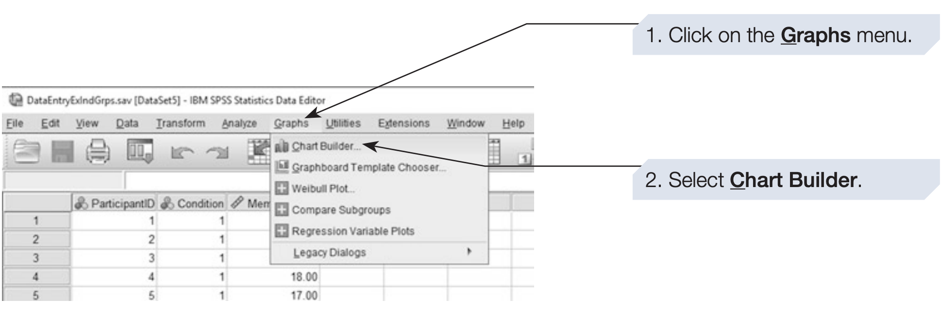
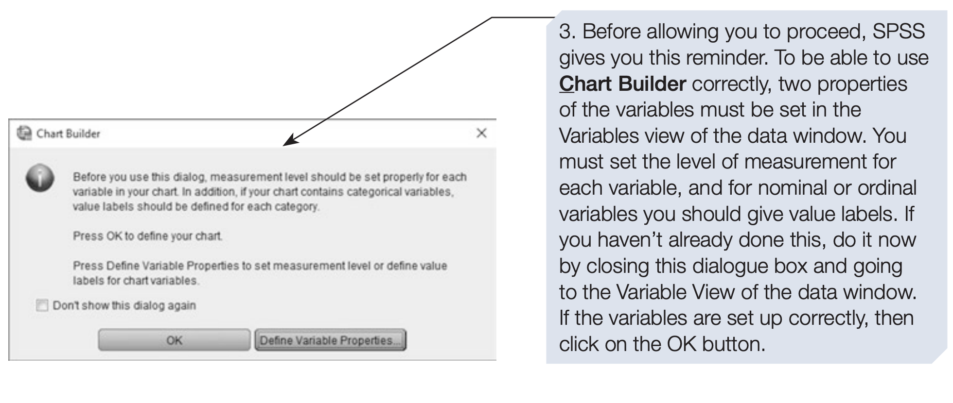
SPSS will open the Chart Builder interface.
Depending on the chart and SPSS version, you can select chart types and specify variables using the Chart Builder.
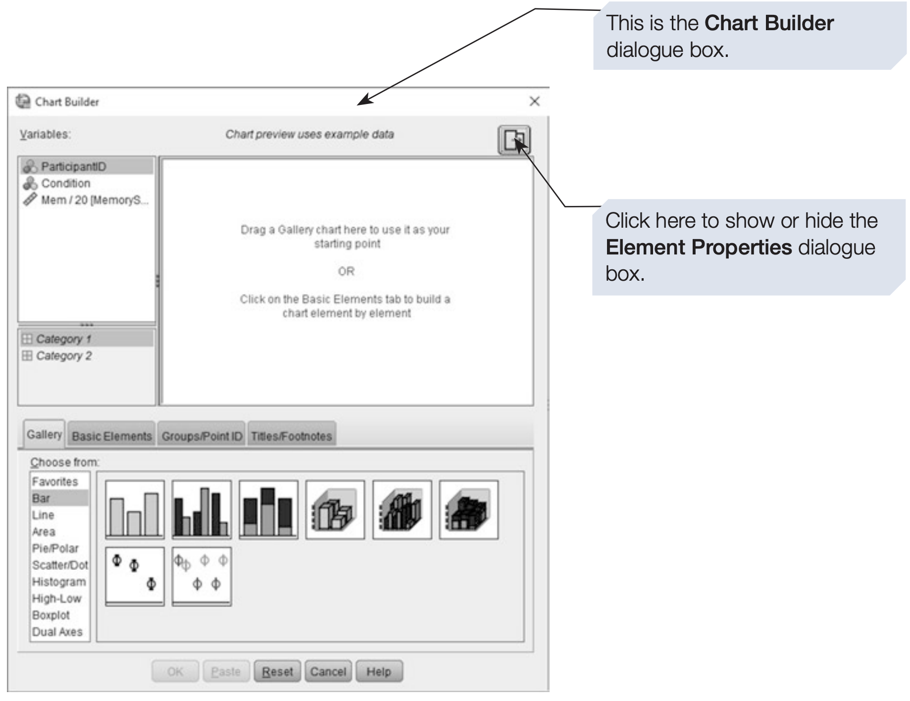
9.1 Element Properties
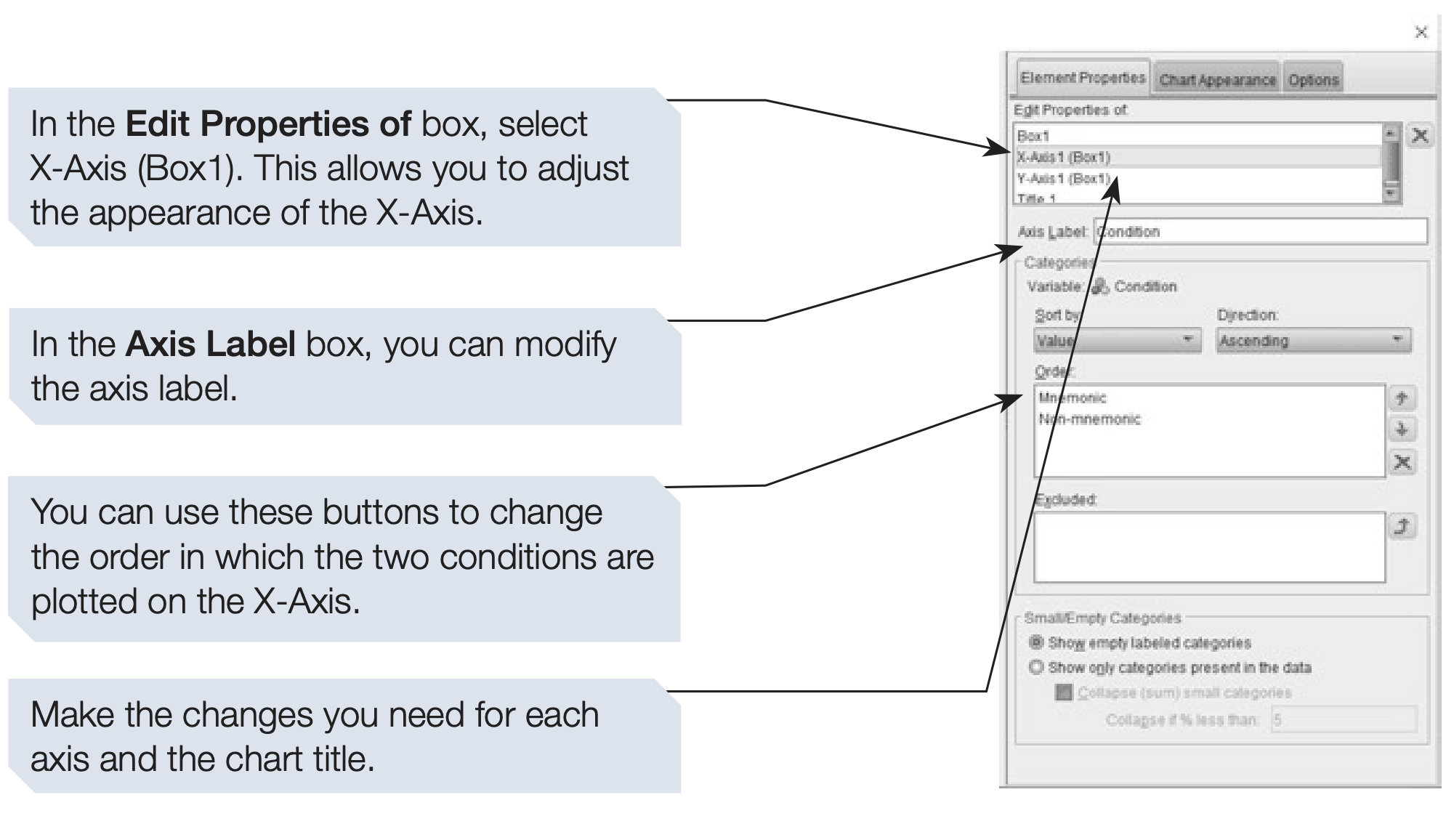
The Element Properties dialog box allows us to modify properties of selected graph elements.
Depending on the graph, we may be able to modify:
- Titles and labels
- Axis scales
- Statistical summaries
- Other graphical properties
After completing the graph specifications, click OK in the Chart Builder dialog box.
The resulting graph will appear in the Viewer window.
9.2 The Graphboard Template Chooser
The Graphboard Template Chooser provides another way to create graphs in SPSS.
It provides a range of templates and can be useful for exploring different visualisations quickly.
Some Graphboard visualisations also support interactive features, depending on the SPSS version.
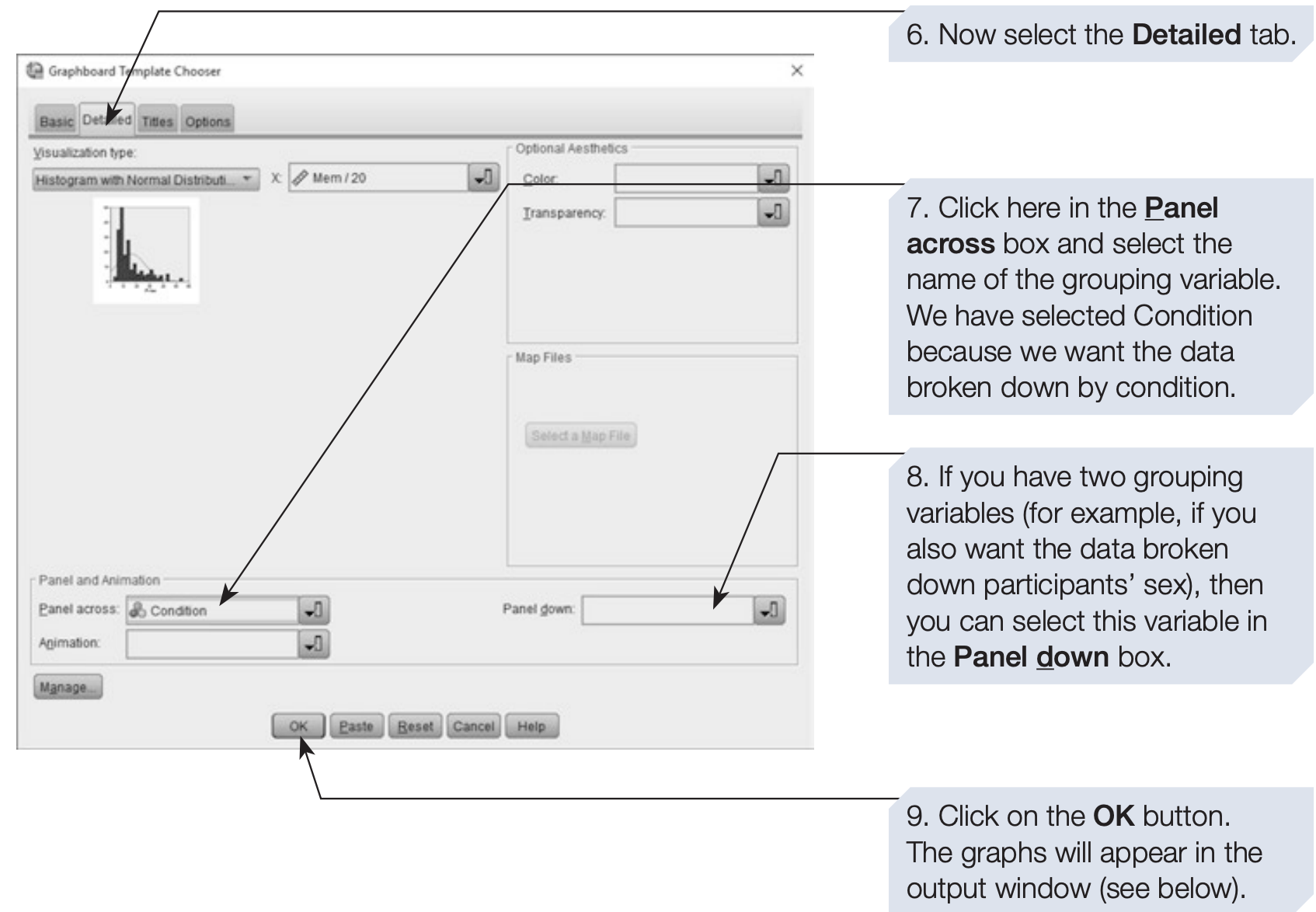
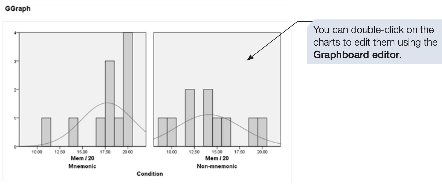
We will illustrate its use by creating histograms for the memory study.
9.3 Steps to Use Graphboard Template Chooser
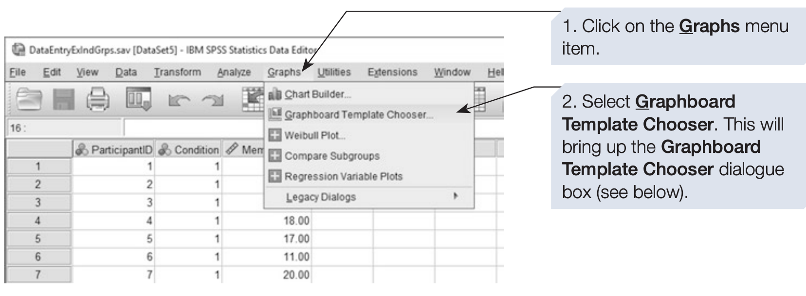
- Click the Graphs menu.
- Select Graphboard Template Chooser.
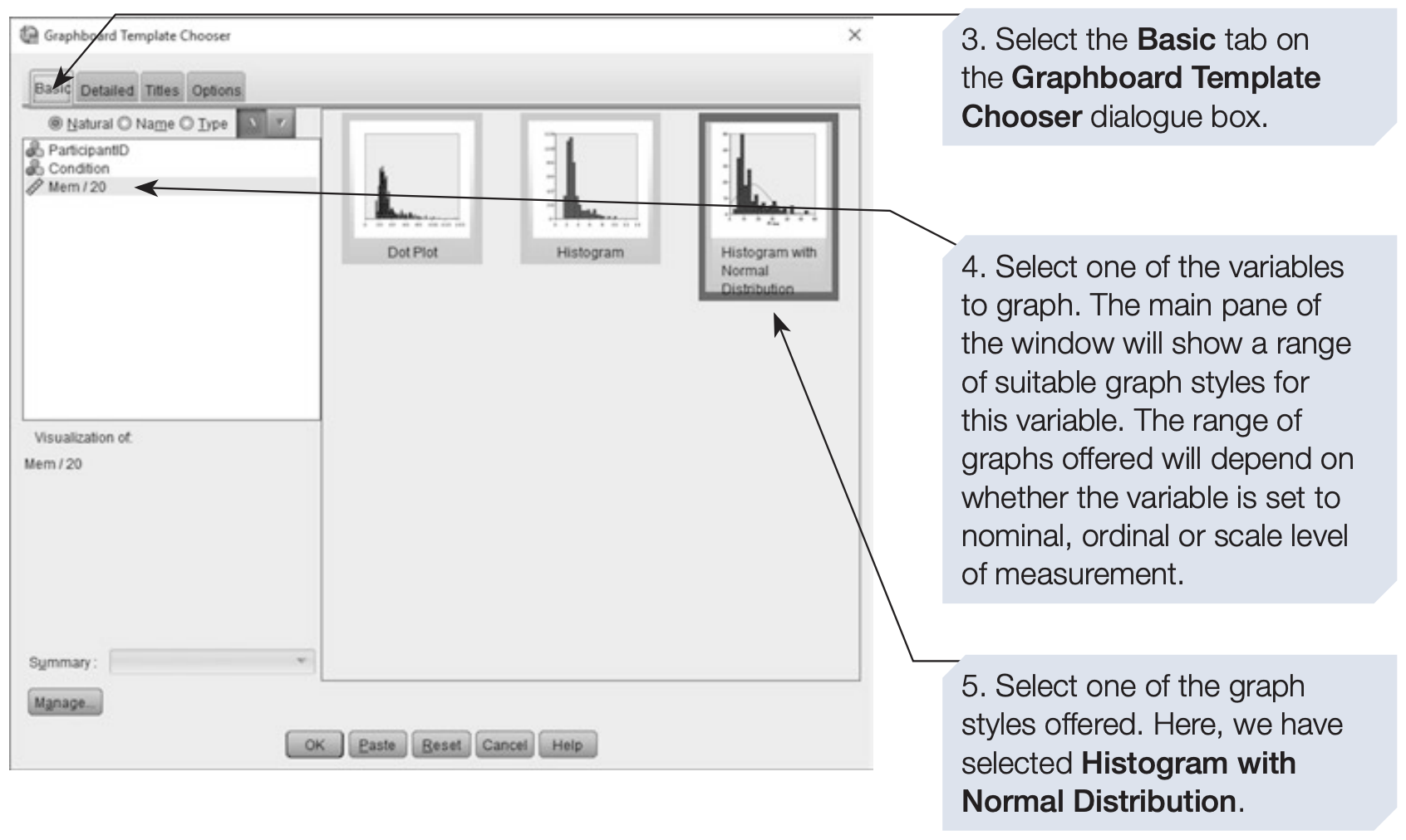
- The following dialog box will appear.
9.4 Editing and Customization
The Graphboard Editor provides options for modifying graphs.
Depending on the graph, you can adjust:
- Titles
- Axis labels
- Legends
- Fonts
- Colours
- Display options
- Other graphical properties
Spend some time exploring these options. The goal is not simply to make graphs attractive, but to make them clear, accurate, and informative.
10 Good Graphs: General Principles
A statistical graph should communicate information clearly rather than simply look attractive.
Give the graph a meaningful title: The reader should understand what the graph shows without needing to guess.
Label the axes: Always make clear:
- What is measured?
- What are the units?
- What do the categories represent?
Choose an appropriate scale: The axis scale should not distort the visual comparison.
Avoid unnecessary decoration: Do not add visual elements that do not communicate information.
Show uncertainty when appropriate: When displaying estimated means or other summaries, consider whether confidence intervals or other uncertainty measures should be shown.
Consider the distribution, not only the mean: A graph of means may hide substantial variation among observations. For quantitative data, boxplots, histograms, and scatterplots can often provide more information than a simple bar chart of means.
Make the graph interpretable without the software: A reader should be able to understand the main message of the graph without knowing how it was produced in SPSS.
11 Summary
Descriptive statistics summarize the main characteristics of data.
Common numerical summaries include:
- Mean, median, and mode.
- Range, IQR, variance, and standard deviation.
- Percentiles and confidence intervals.
SPSS provides several procedures for descriptive analysis, including:
- Descriptives
- Frequencies
Graphs can reveal patterns that may not be obvious from numerical summaries alone.
Boxplot → summarizes a quantitative distribution and is useful for comparing groups and identifying potential outliers.
Histogram → shows the distribution of a quantitative variable.
Bar chart → compares frequencies, percentages, or summary statistics across categories.
Scatterplot → displays the relationship between two quantitative variables.
Key principle: Choose a graph based on the type of data and the question you want the graph to answer, not simply on which graph looks most attractive.
| Purpose | Suitable graph |
|---|---|
| Distribution of a quantitative variable | Histogram |
| Compare distributions across groups | Boxplot |
| Frequencies of categories | Bar chart |
| Examine relationship between two quantitative variables | Scatterplot |