4 Data Handling

(PSY206) Data Management and Analysis

Author

Md Rasel Biswas

SPSS provides a range of commands to modify, manipulate, or transform data, collectively referred to as Data Handling commands.
These commands are particularly useful when working with large datasets containing numerous variables for each participant, such as survey or questionnaire data.
Questionnaires often include items (questions) that can be grouped into subscores, which can be calculated using Data Handling commands.
Data transformations, such as log transformations, can also be performed to reduce distortions like skewness and improve the validity of statistical analyses.
Another common use of these commands is to filter data to analyze specific groups of participants — for example, analyzing males and females separately, or excluding respondents who do not meet certain inclusion criteria.

Example Data File

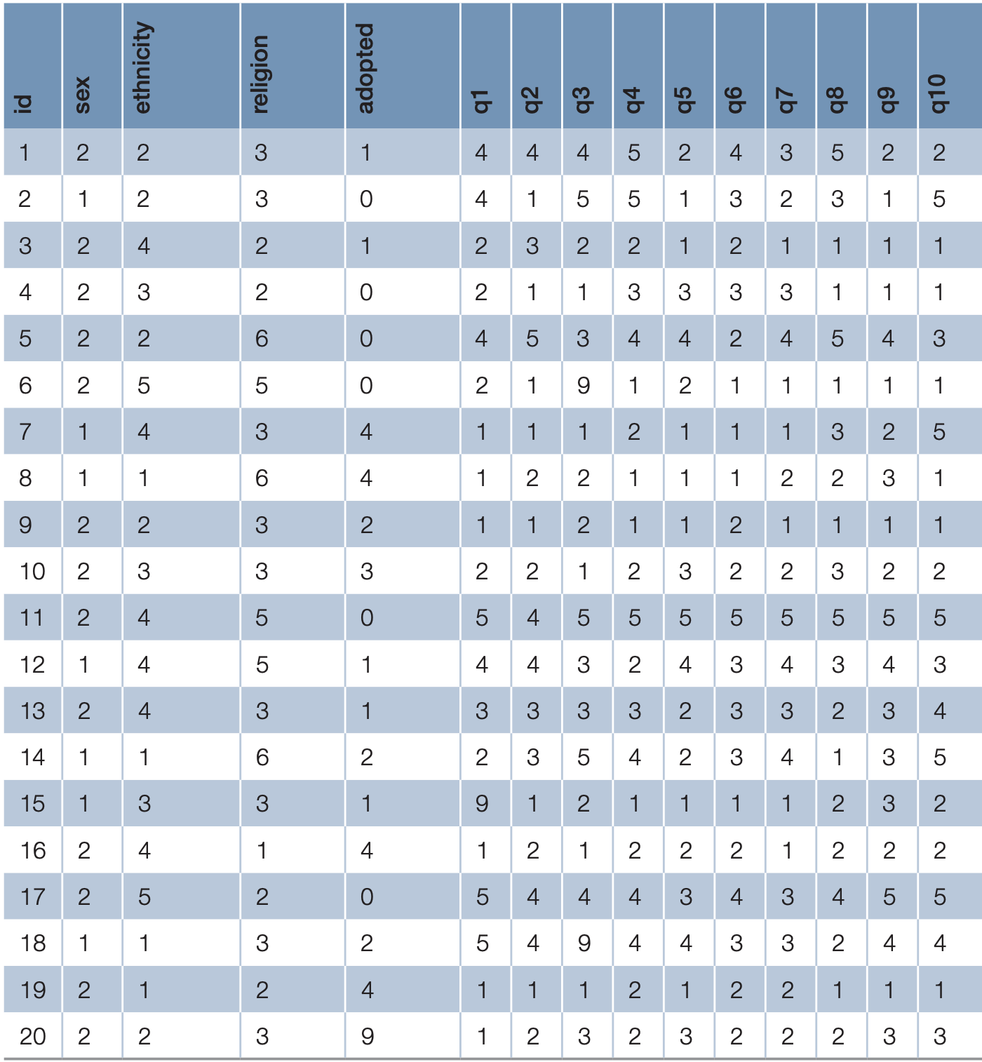
To illustrate the use of these commands, we will use a small dataset (download adoption_survey.xlsx) based on a fictitious survey exploring people’s attitudes toward adoption.

This dataset includes:

Participant number
Demographic variables (age, sex, ethnicity, religious belief, and adoption experience)
Responses to 10 statements on adoption, measured on a 5-point Likert scale ranging from Strongly Agree (1) to Strongly Disagree (5)

Each response is recorded in variables q1 to q10.

SPSS syntax: importing the example data

/* Import the adoption survey from Excel */
GET DATA
  /TYPE=XLSX
  /FILE='C:\your\folder\adoption_survey.xlsx'
  /SHEET=name 'Sheet1'
  /CELLRANGE=FULL
  /READNAMES=ON.

EXECUTE.

/* Optional: add variable labels. */
VARIABLE LABELS
  id        'Participant ID'
  sex       'Sex'
  ethnicity 'Ethnicity'
  religion  'Religion'
  adopted   'Adoption experience'
  q1        'Q1: attitude statement 1'
  q2        'Q2: attitude statement 2'
  q3        'Q3: attitude statement 3'
  q4        'Q4: attitude statement 4'
  q5        'Q5: attitude statement 5'
  q6        'Q6: attitude statement 6'
  q7        'Q7: attitude statement 7'
  q8        'Q8: attitude statement 8'
  q9        'Q9: attitude statement 9'
  q10       'Q10: attitude statement 10'.

EXECUTE.

4.1 Sorting Data

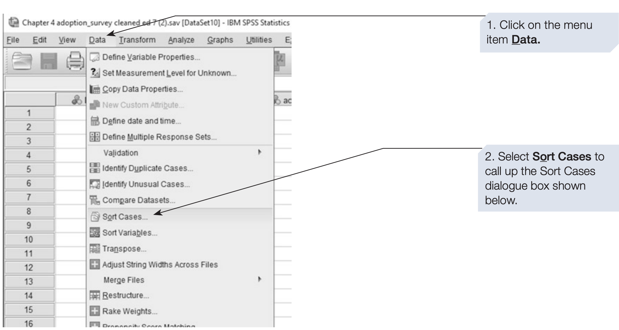
Although the order of cases usually does not affect statistical analysis, sorting can make it easier to inspect and verify data. For example, sorting participants by sex and then by ethnicity can help detect data entry issues or compare group distributions.

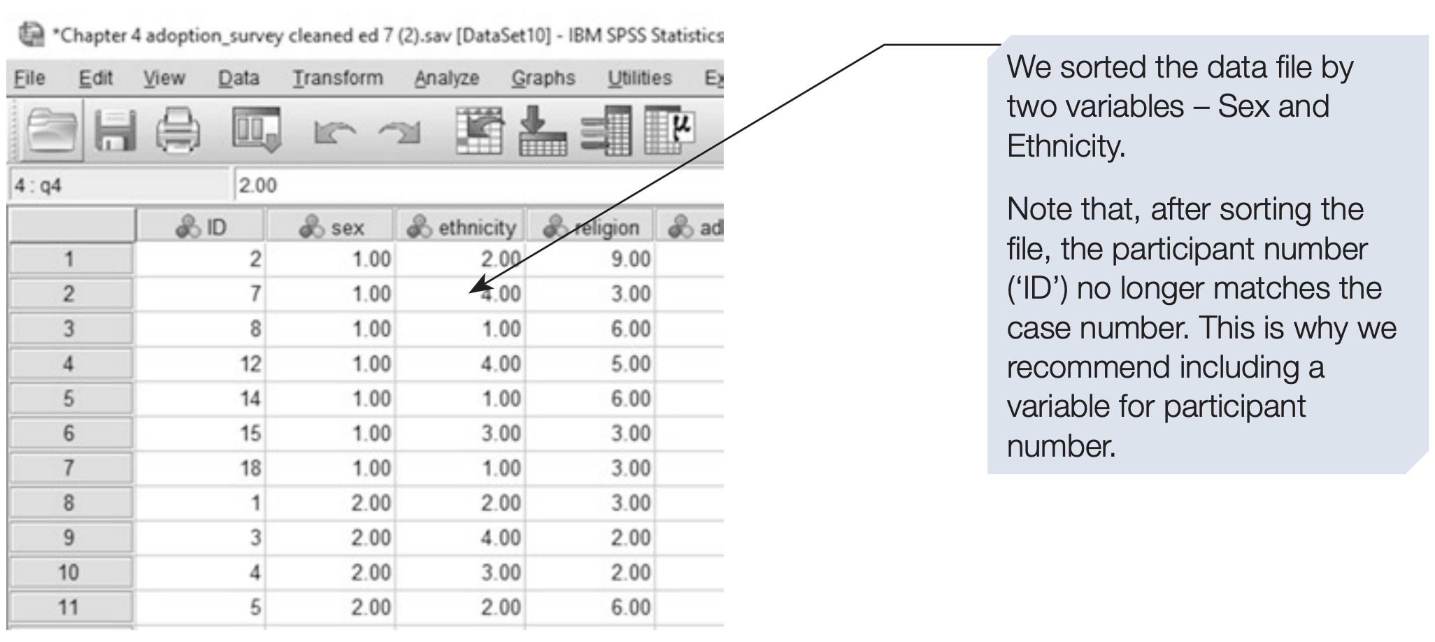
In this example, we sort the data first by sex, and then within each sex by ethnicity.

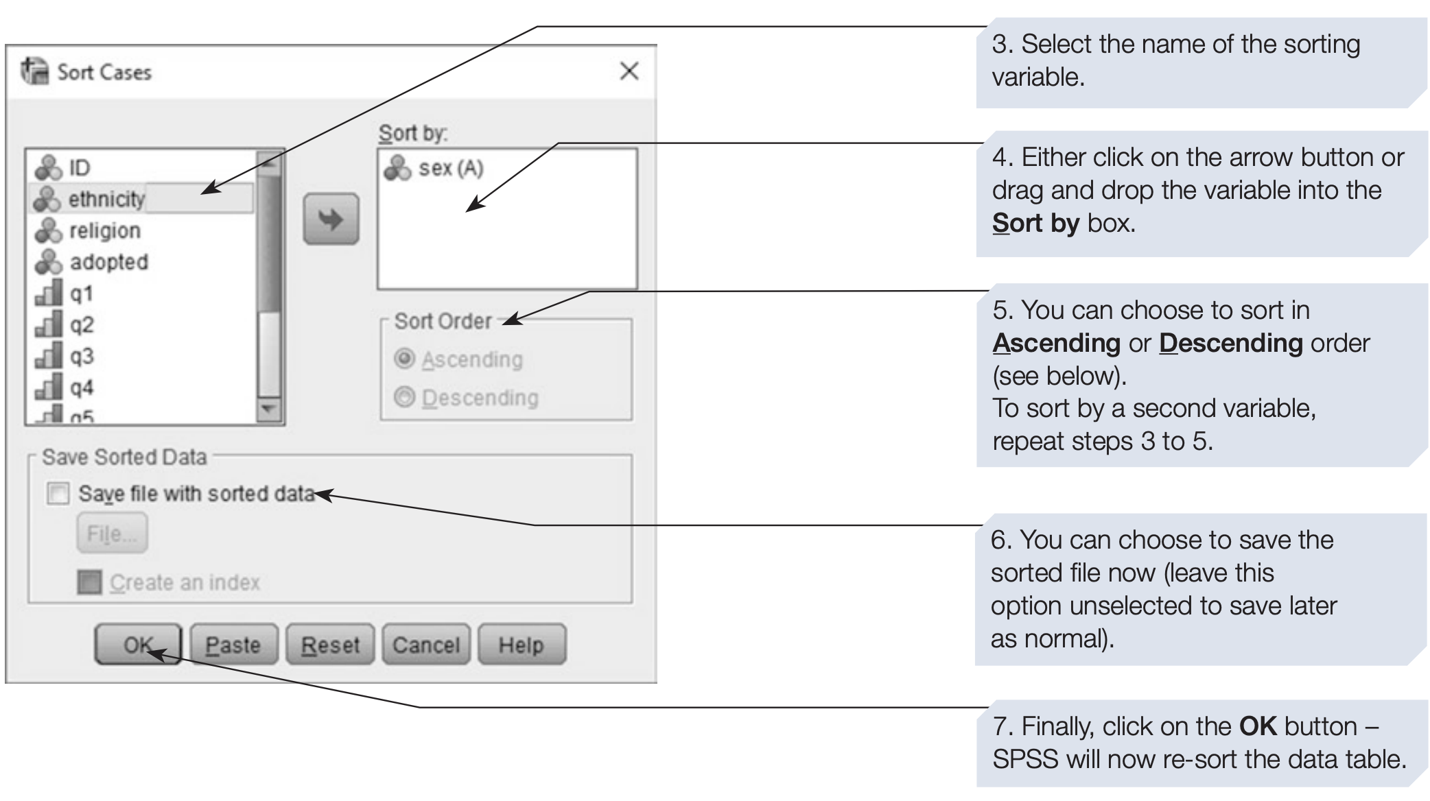
SPSS syntax: sorting by sex and ethnicity

/* Sort cases first by sex, then by ethnicity */
SORT CASES BY sex (A) ethnicity (A).
EXECUTE.

4.2 Splitting Data

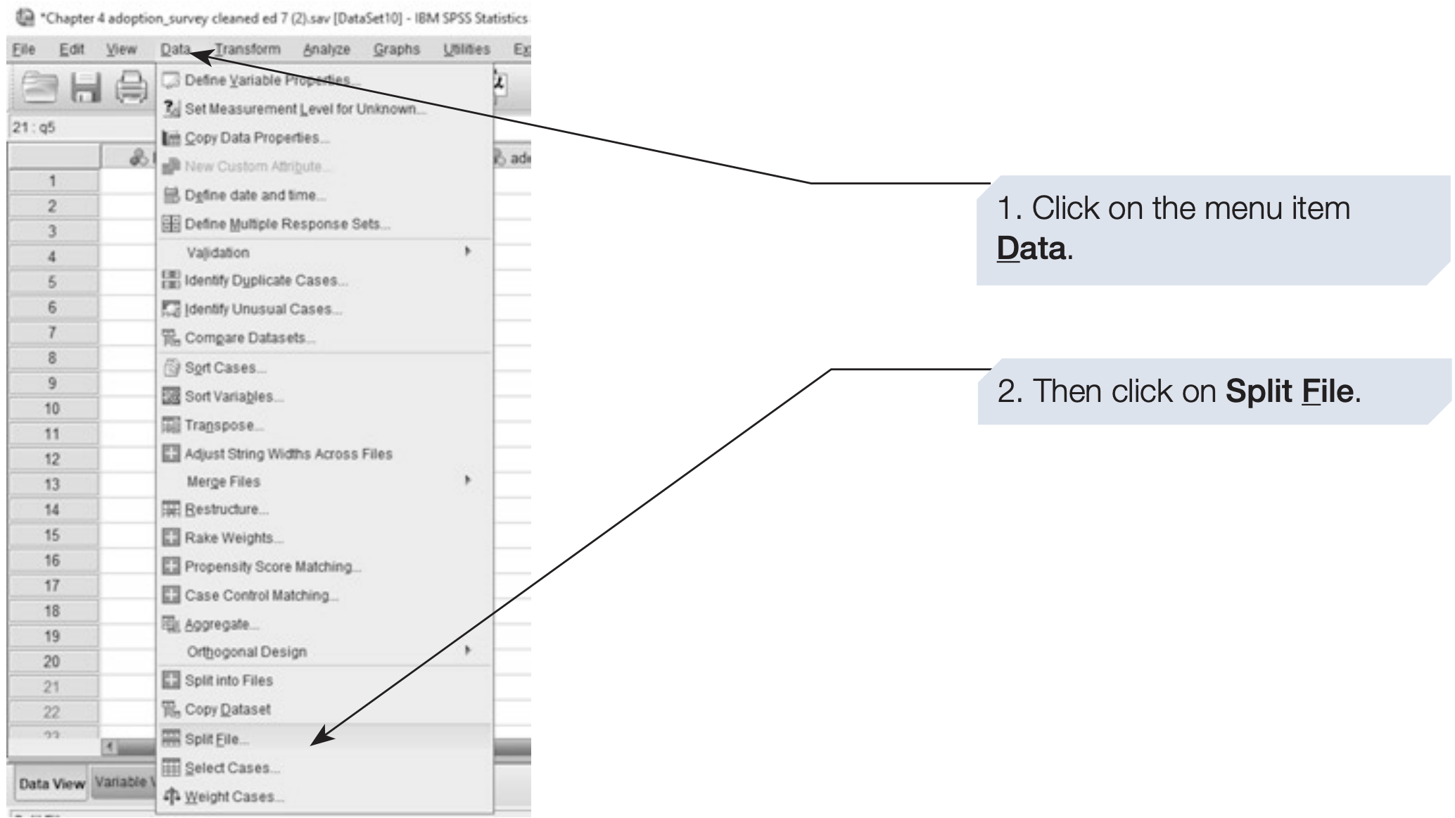
The Split File function allows SPSS to temporarily divide a dataset into groups, so that all subsequent analyses are performed separately for each group.

For instance, you may want to produce separate statistical outputs for male and female participants.

To split a file, follow the steps below:

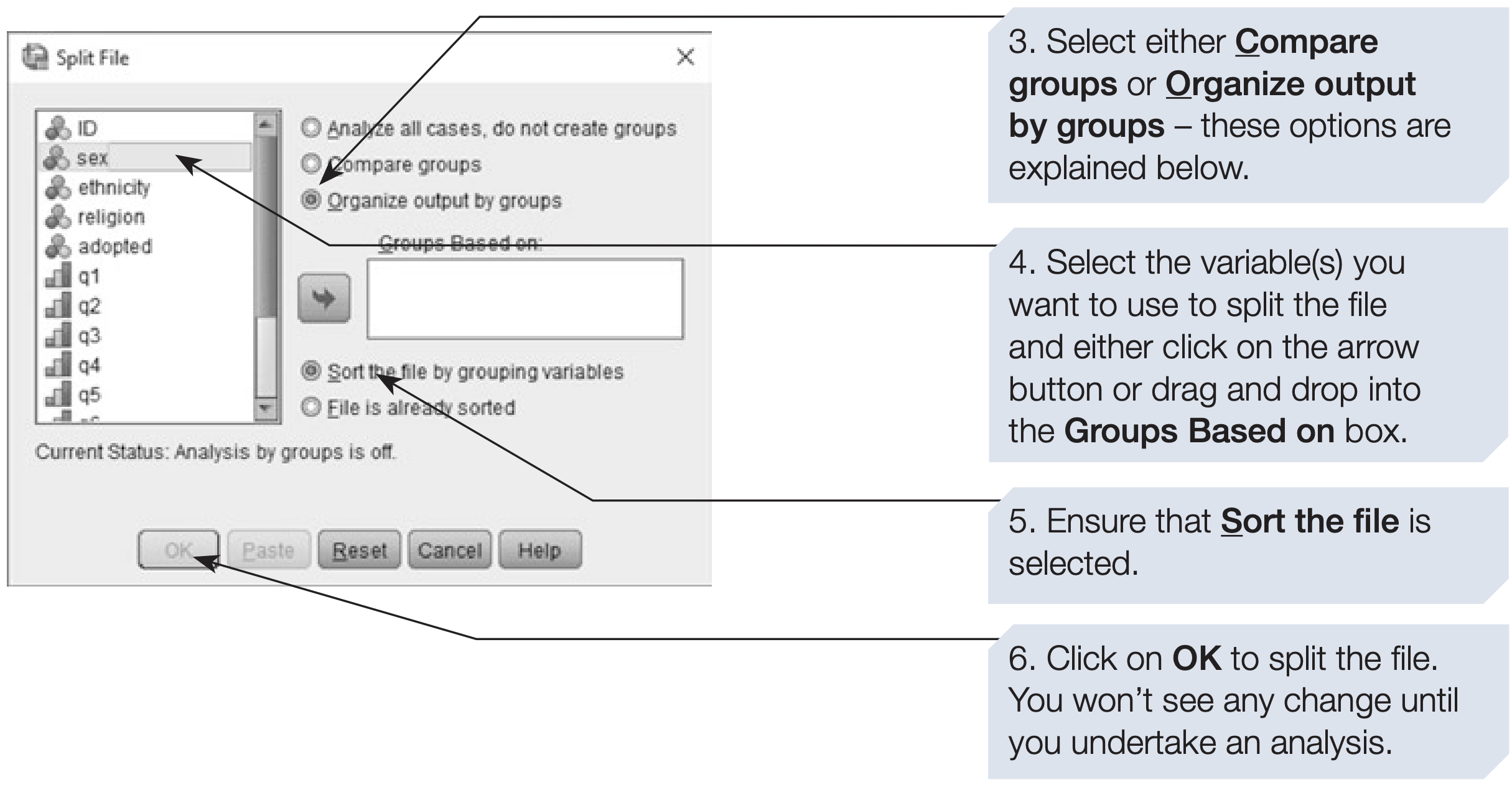
The difference between the two options is important:

Compare groups: produces one combined output section showing group comparisons.
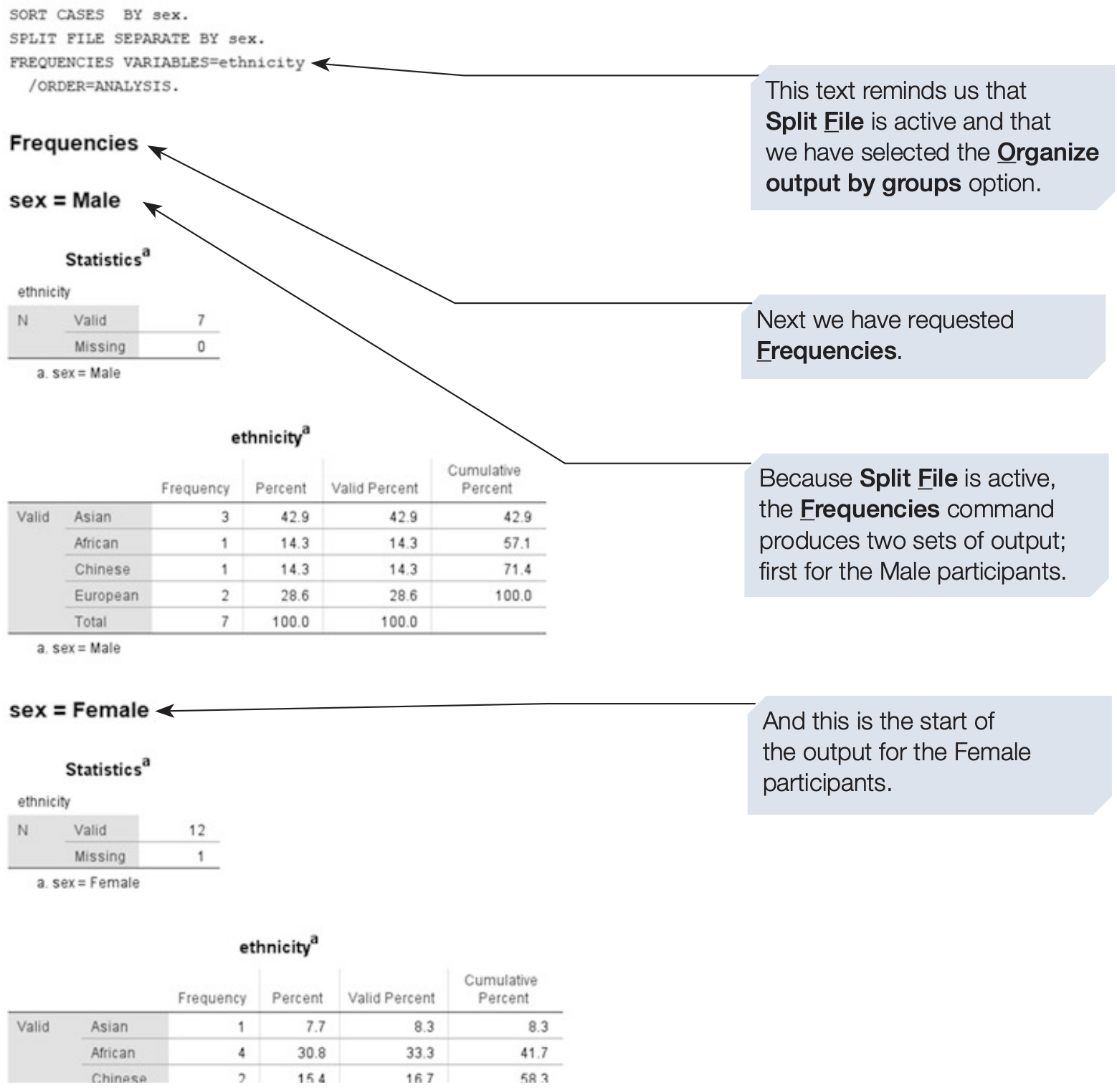
Organize output by groups: generates separate output sections for each group.

We usually prefer Organize output by groups for clearer interpretation, but you should explore both options to understand their differences.

SPSS syntax: splitting the file by sex

/* Run analyses separately for each level of sex. */
SPLIT FILE LAYERED BY sex.

/* Example: descriptive statistics for q1–q10 by sex. */
DESCRIPTIVES VARIABLES=q1 TO q10
  /STATISTICS=MEAN STDDEV MIN MAX.

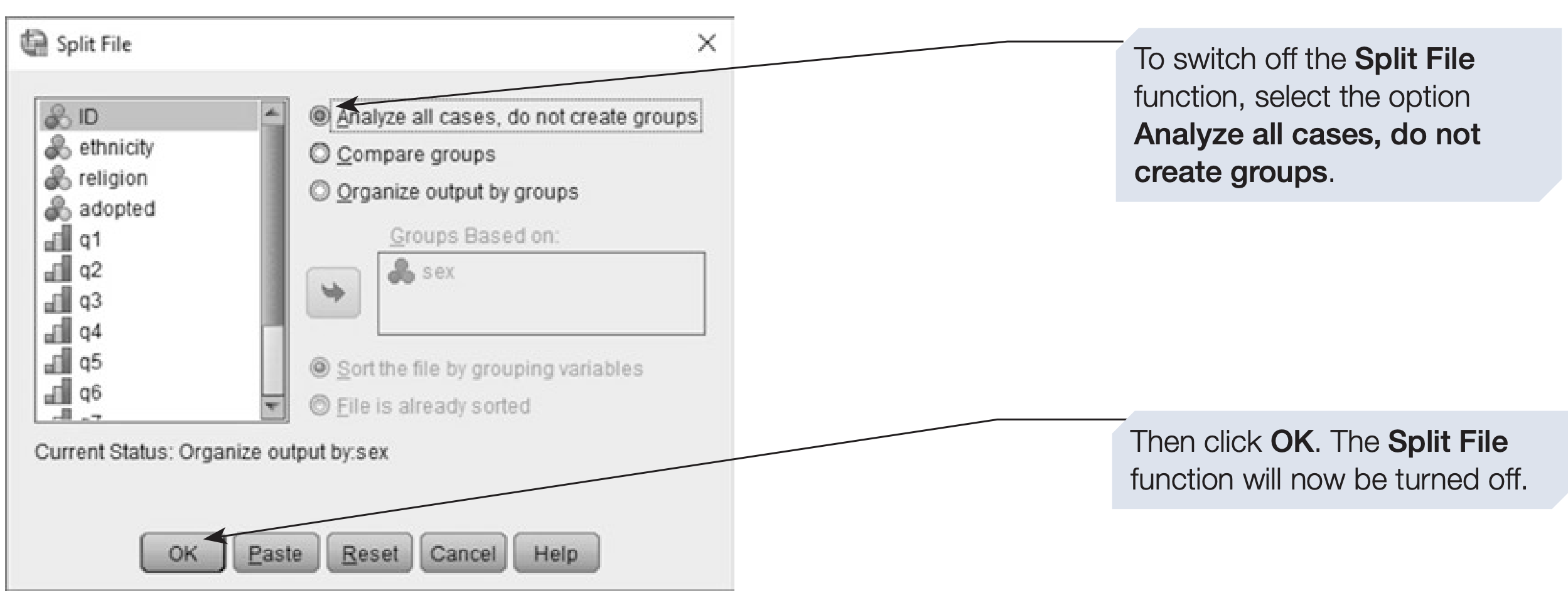
/* Remember to turn Split File off when finished (see below). */

Undoing Split File

The Split File command remains active until you manually turn it off. You can check whether it is on by looking at the bottom-right corner of the Data View window. When Split File is active, SPSS displays a message like “Split by Sex.”

To disable it, simply select Unsplit File from the same menu.

SPSS syntax: turning Split File off

/* Turn off Split File. */
SPLIT FILE OFF.
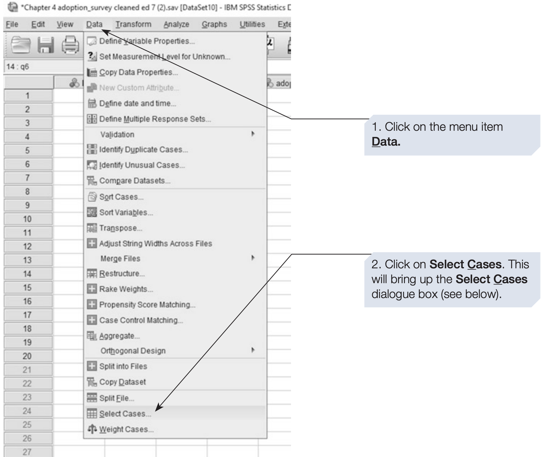
EXECUTE.

4.3 Selecting Cases

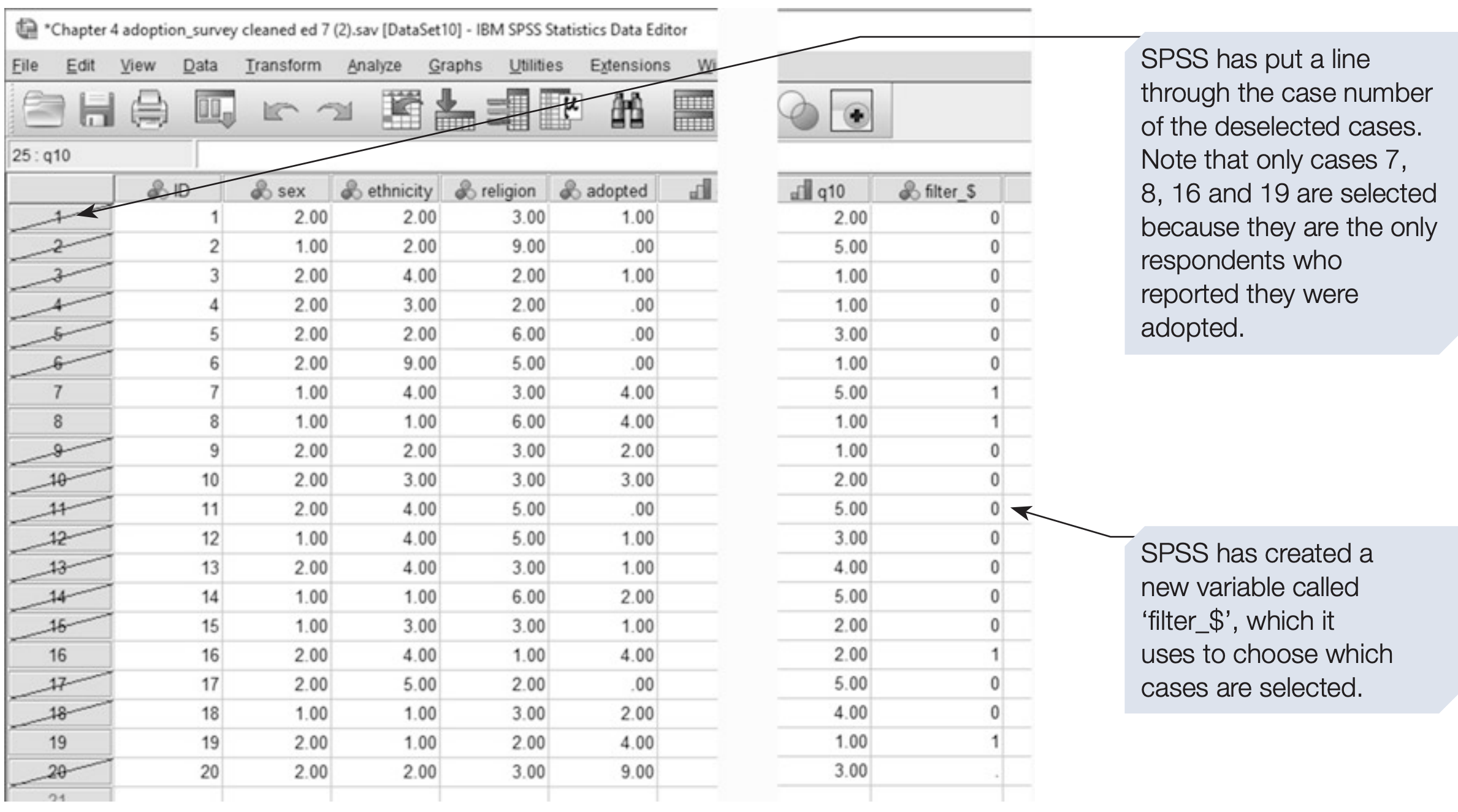
Sometimes you may wish to analyze only a subset of your data, such as respondents who have been adopted.
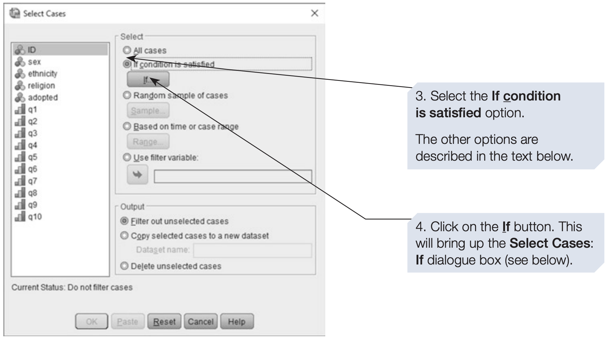
The Select Cases command allows you to temporarily exclude all other participants from analysis.

Split File analyzes all data but displays separate outputs by group.
Select Cases analyzes only the chosen subset, suppressing all other cases.

Use Select Cases when you want to restrict analysis to specific participants.

SPSS syntax: selecting only participants with adoption experience

/* Keep only cases with some adoption experience (adopted > 0). */
USE ALL.
COMPUTE filter_$ = (adopted > 0).
FILTER BY filter_$.
EXECUTE.

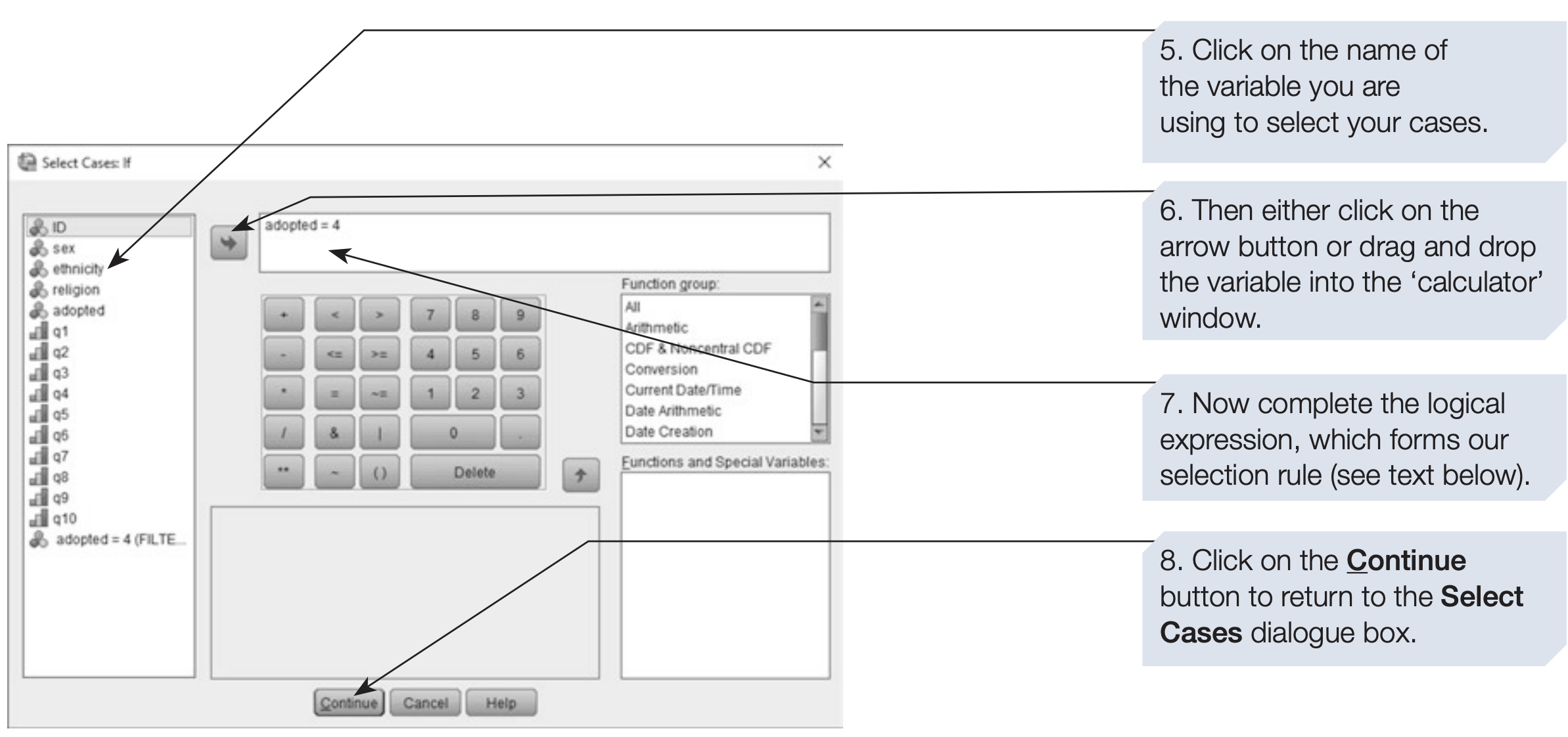
* All subsequent analyses now use only cases with adopted > 0.

Selection Rules

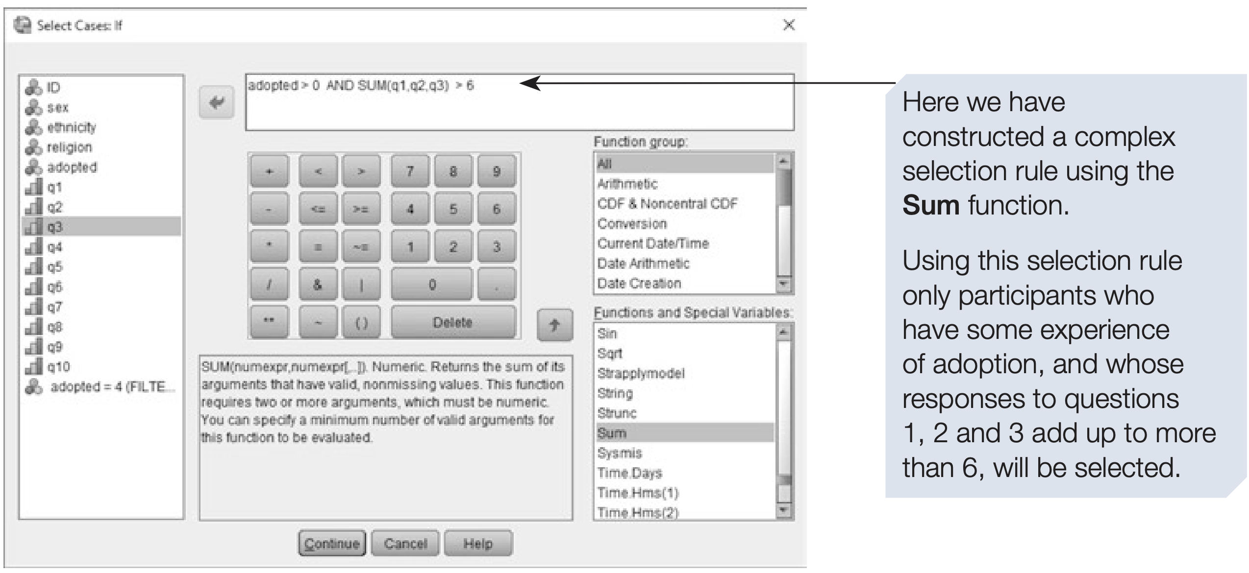
You can define complex selection criteria using logical operators such as AND, OR, and NOT.
Rules can be typed directly or created using the on-screen calculator.

For example, to select only Chinese Christians with experience of adoption, the expression would be: religion = 3 and ethnicity = 3 and adopted > 0

You can also create more advanced selection rules by combining logical conditions with built-in functions available in the dialogue box.

SPSS syntax: complex selection with logical operators

/* Select Chinese Christians with adoption experience. */
USE ALL.
COMPUTE filter_$ = (religion = 3 AND ethnicity = 3 AND adopted > 0).
FILTER BY filter_$.
EXECUTE.

Reselecting All Cases

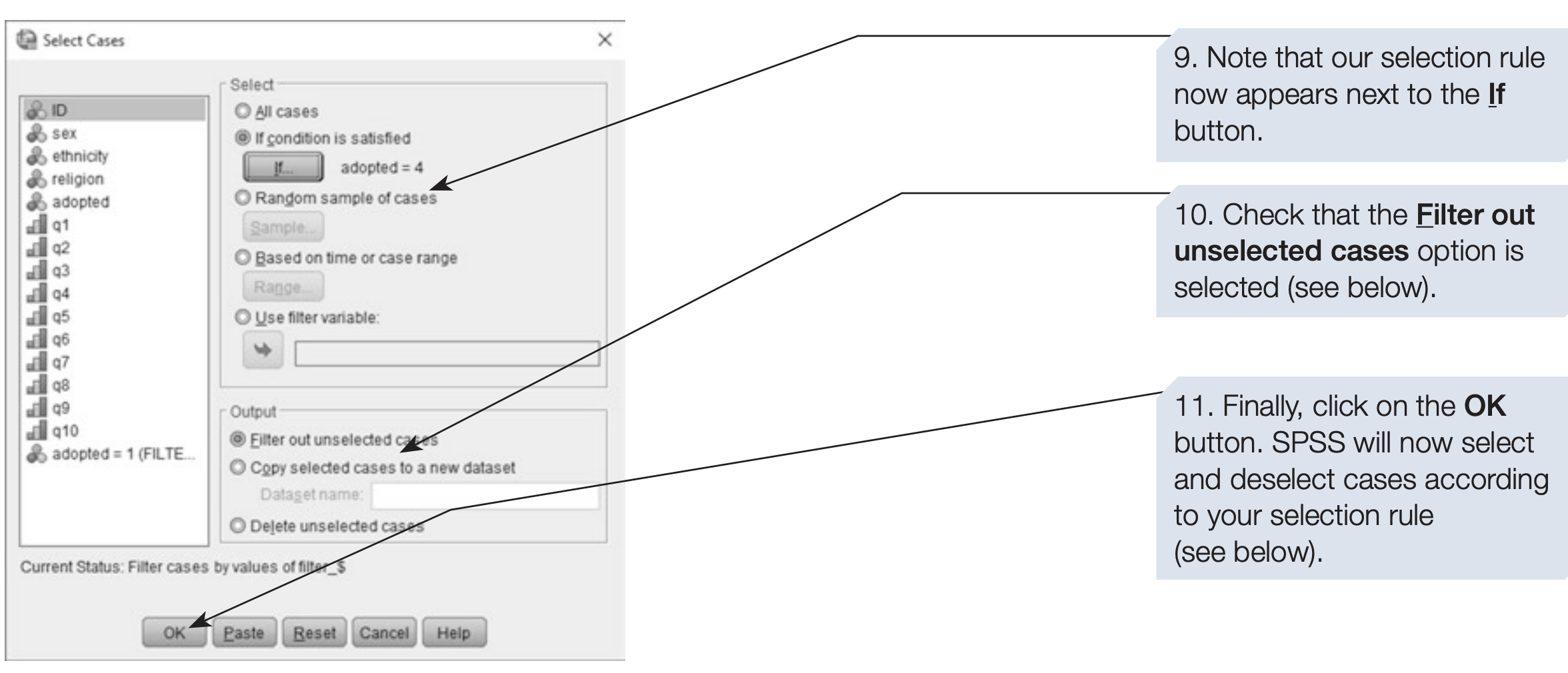
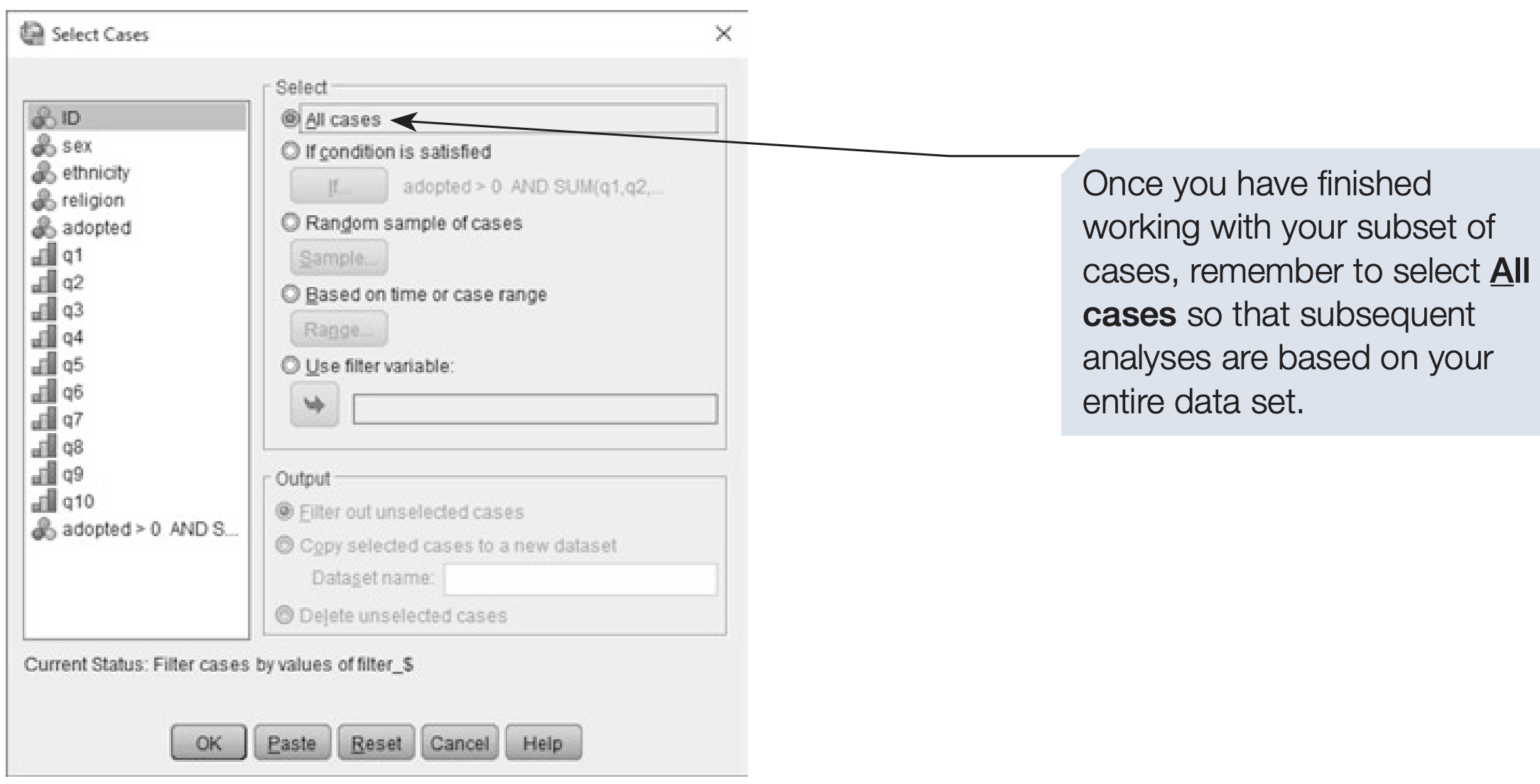
The selection remains in effect until you manually reset it.
To restore all participants, open the Select Cases dialog and choose All cases.

SPSS syntax: restoring all cases

/* Turn off the filter and include all participants again. */
FILTER OFF.
USE ALL.
EXECUTE.

4.4 Recoding Values

Recoding is the process of changing the values of a variable — often to correct errors, merge categories, or prepare data for specific analyses.

For instance, if preliminary results show very few participants with adoption experience through “immediate family” or “other family,” these categories could be combined.

SPSS provides two main recode options:

Recode into Same Variables — replaces original values (riskier)
Recode into Different Variables — creates a new variable (safer and recommended)

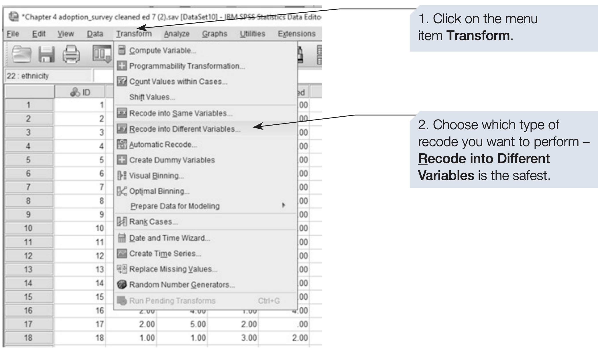
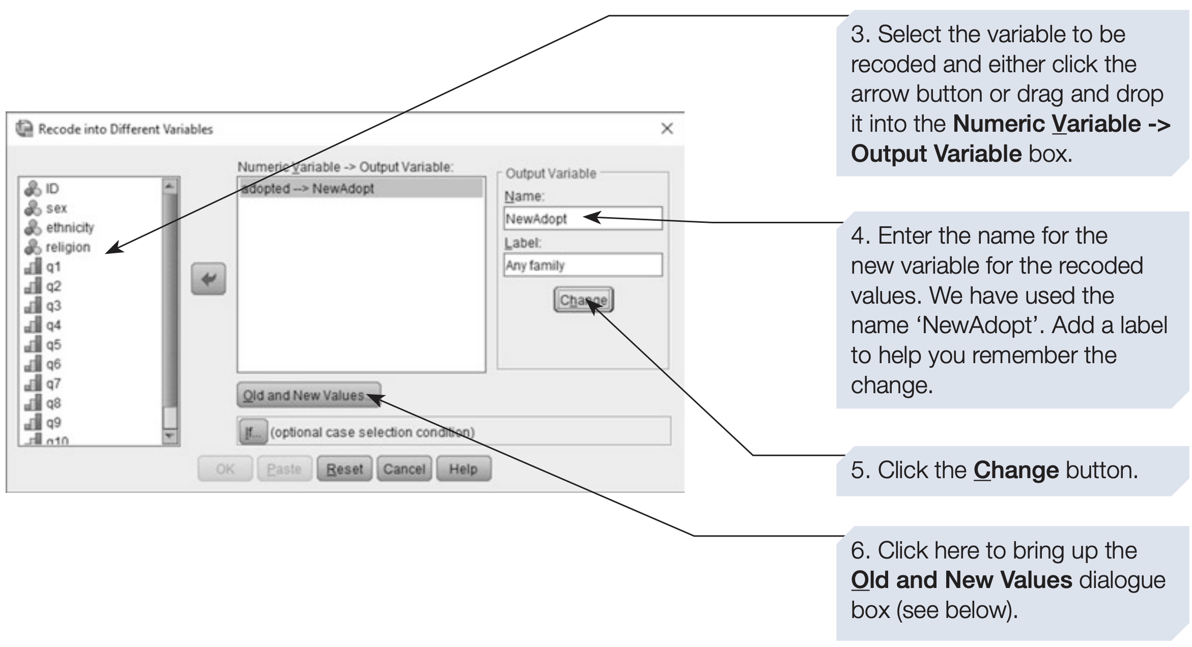
Tip: Always use Recode into Different Variables to preserve the original data in case of mistakes.

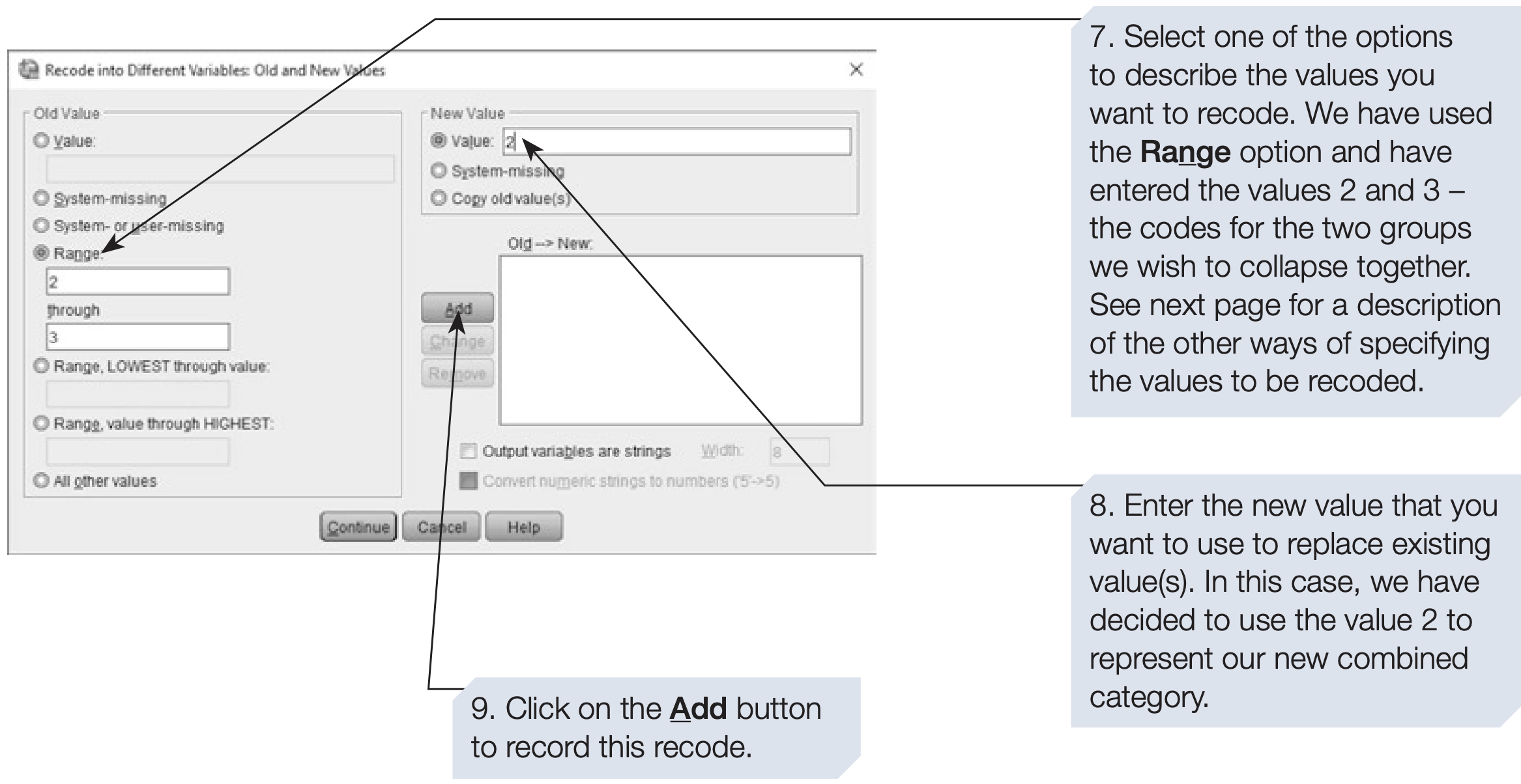
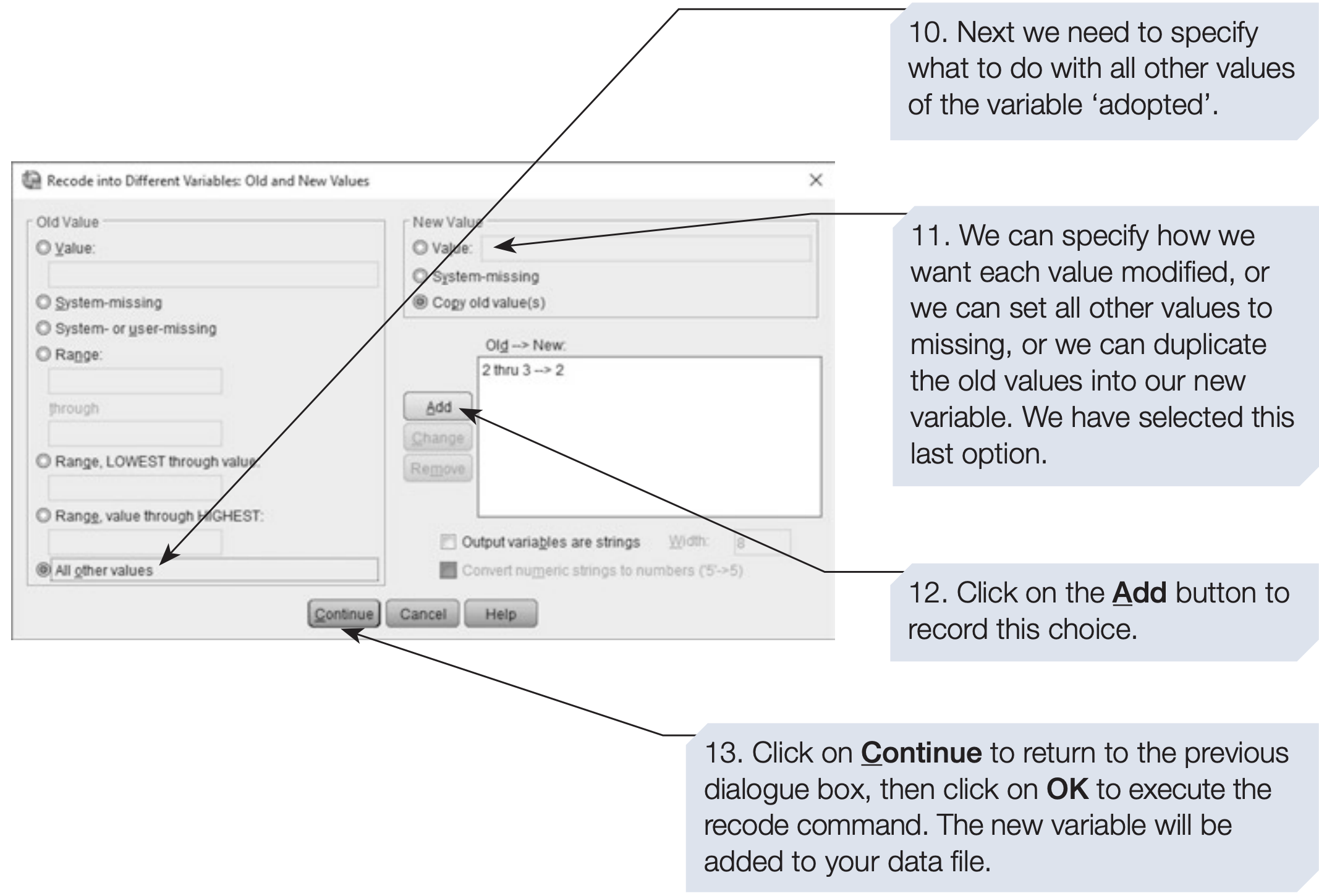
SPSS syntax: recoding adoption experience

/* Recode adopted into a simpler binary variable by combining 2 and 3 */

RECODE adopted (2,3 = 2) INTO NewAdopt.
EXECUTE.

Conditional Recoding

You can also apply conditional recoding, where values are changed only if specific conditions are met — for example, recoding age values only for female participants.

This can be achieved by using the If button, which appears in both the Recode into Different Variables and the Recode into Same Variables dialogue boxes.

SPSS syntax: conditional recoding example

/* Example: reverse-score q1 only for female participants (sex = 2).
   Original scale: 1 = Strongly Agree ... 5 = Strongly Disagree. */

IF (sex = 2) q1_rev = 6 - q1.
VARIABLE LABELS q1_rev 'Q1 (reverse-scored for females only)'.

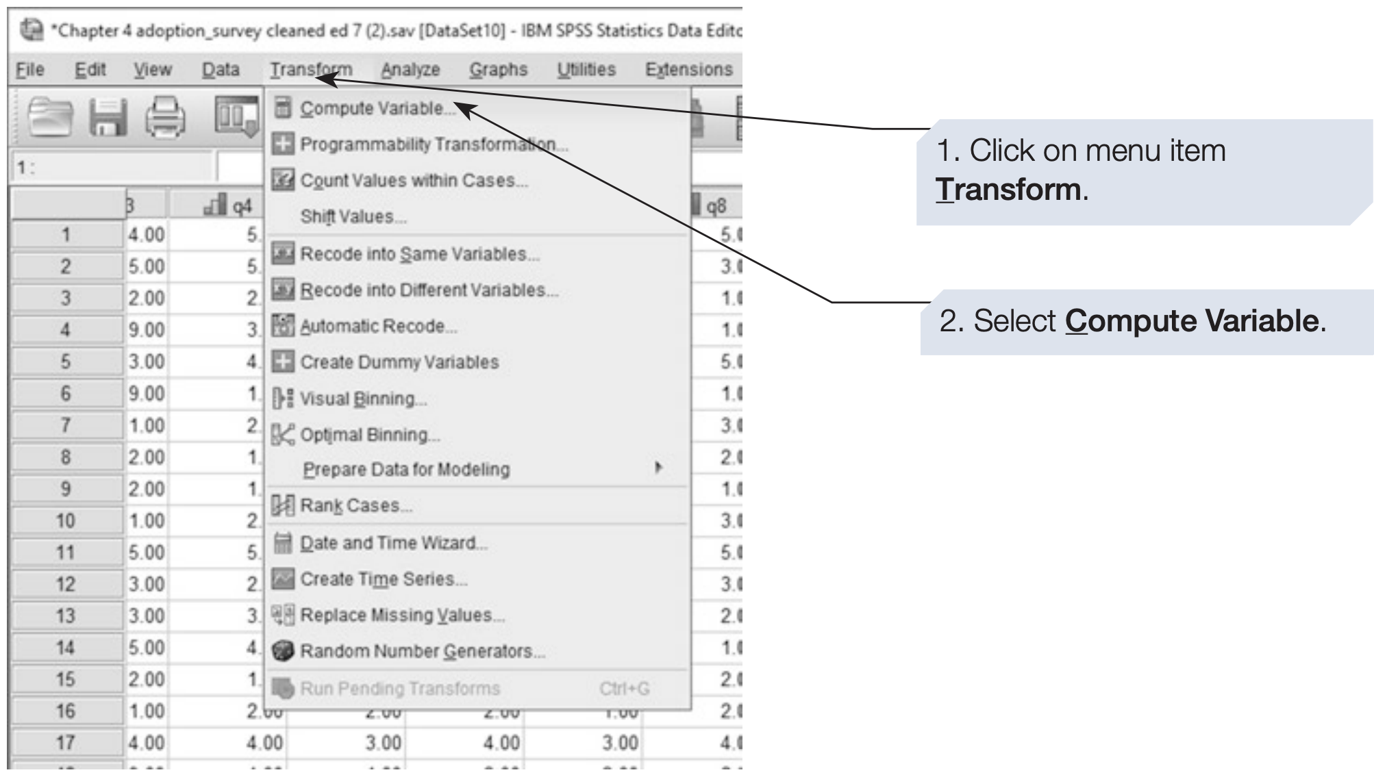
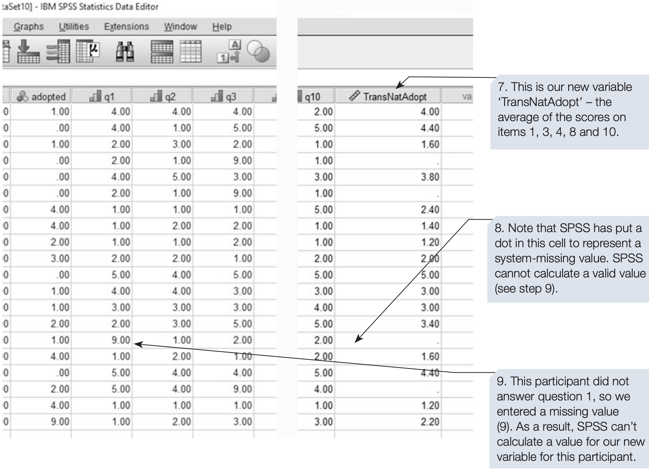
EXECUTE.

4.5 Computing New Variables

The Compute Variable command allows you to create new variables from existing ones.
This is useful when:

Summing item scores into total or subscale scores
Calculating averages
Applying mathematical transformations

In our example, the 10 questionnaire items can be combined into two subscales by summing or averaging specific variables (q1–q5, q6–q10).

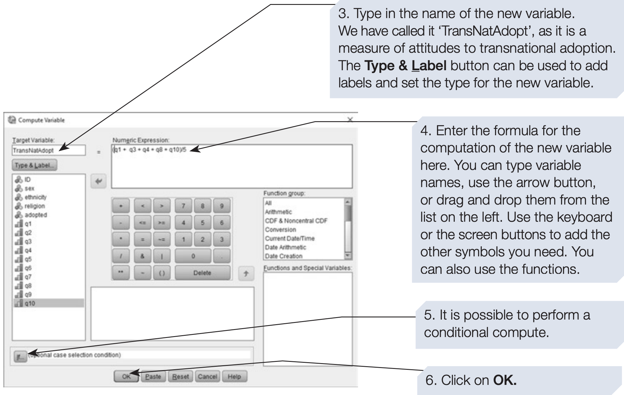
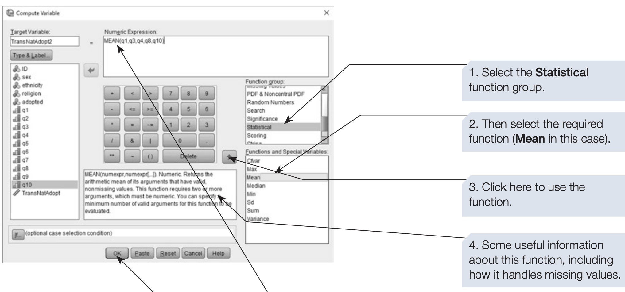
SPSS also provides built-in functions such as SUM(), MEAN(), SD(), etc., that simplify computation.

SPSS syntax: computing subscale and total scores

/* Subscale 1: sum of q1–q5. */
COMPUTE adopt_sub1 = SUM(q1 TO q5).

/* Subscale 2: sum of q6–q10. */
COMPUTE adopt_sub2 = SUM(q6 TO q10).

/* Total attitude score across all 10 items (mean score). */
COMPUTE adopt_total_mean = MEAN(q1 TO q10).

VARIABLE LABELS
  adopt_sub1      'Adoption attitude subscale 1 (q1–q5)'
  adopt_sub2      'Adoption attitude subscale 2 (q6–q10)'
  adopt_total_mean 'Adoption attitude total (mean of q1–q10)'.

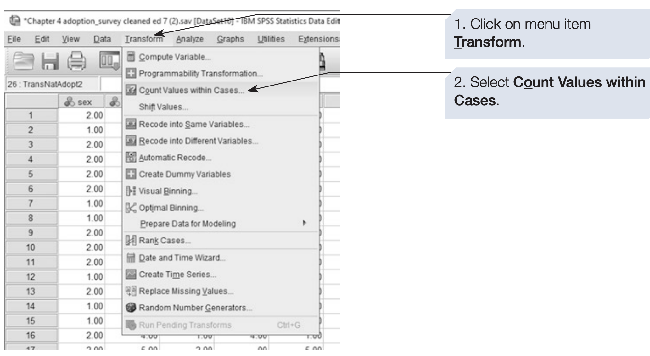
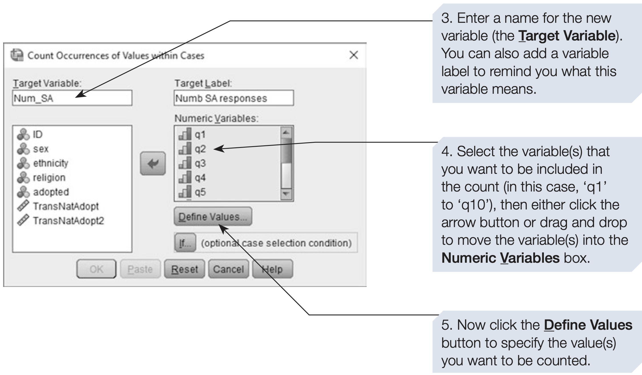
EXECUTE.

4.6 Counting Values

Sometimes we need to count how many times a particular response occurs across several variables.
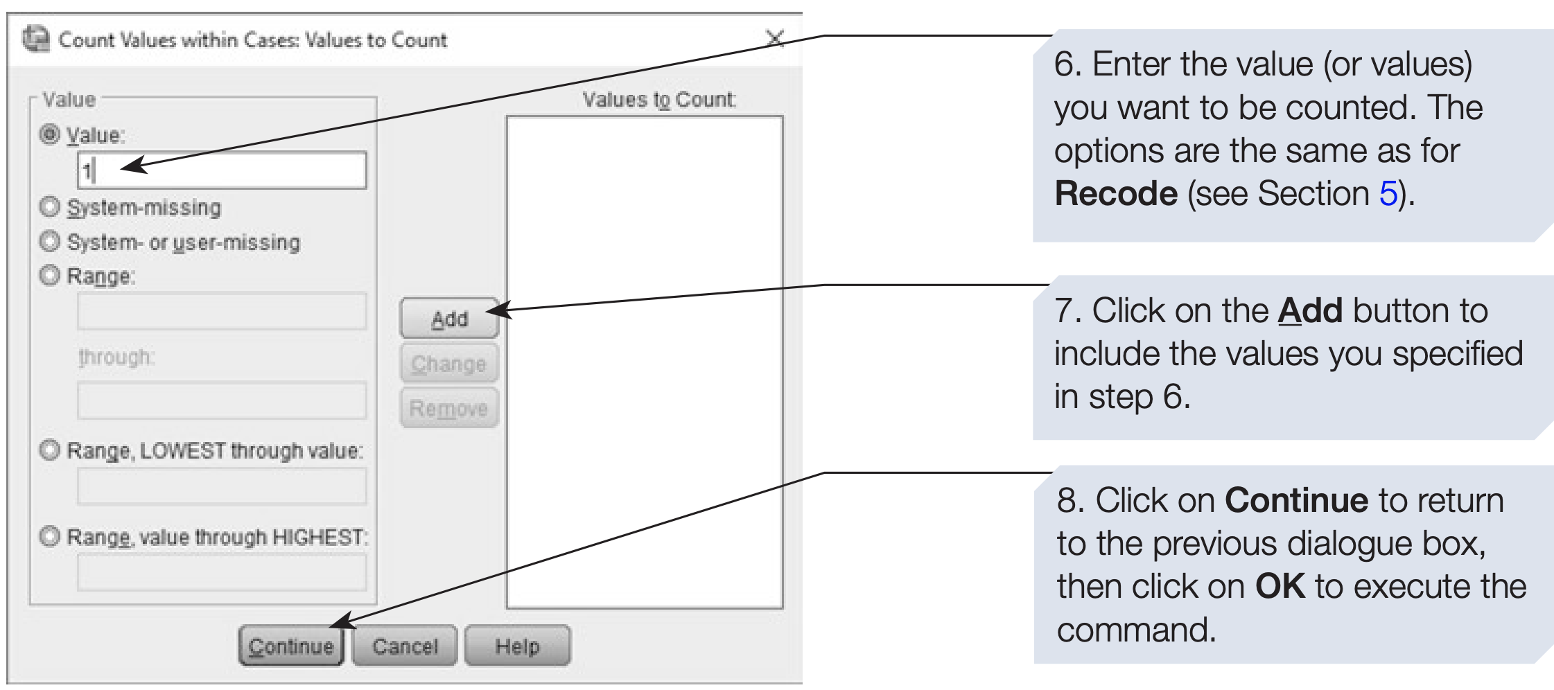
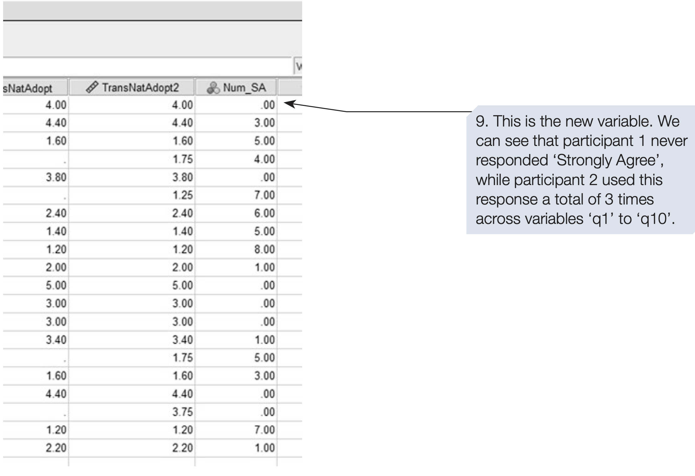
For example, you may want to know how many times each participant selected “Strongly Agree (1)” across all 10 questionnaire items (q1–q10).

The Count Values within Cases function creates a new variable representing this count.

SPSS syntax: counting “Strongly Agree (1)” responses

/* Count how many times each participant answered 1 (Strongly Agree)
   across items q1–q10. */

COUNT strong_agree = q1 TO q10 (1).
VARIABLE LABELS strong_agree 'Number of Strongly Agree responses (1) across q1–q10'.

EXECUTE.

Summary

In this chapter, you learned how to:

Sort and split datasets
Select specific cases for analysis
Recode and compute variables
Count responses across variables

These data handling skills are fundamental for data preparation and cleaning — an essential step before conducting any statistical analysis in SPSS.

Here is a clean, compact Summary Table of SPSS Data-Handling Syntaxes that you can paste directly into your .qmd or .md file.

Summary of SPSS Syntax

1. Importing Data

Import Excel file

GET DATA
  /TYPE=XLSX
  /FILE='path\adoption_survey.xlsx'
  /SHEET=name 'Sheet1'
  /READNAMES=ON.
EXECUTE.

Add variable labels
```
VARIABLE LABELS var 'Label'.
EXECUTE.
```

2. Sorting Data

Sort by sex, then ethnicity

SORT CASES BY sex (A) ethnicity (A).
EXECUTE.

3. Splitting Data

Split analyses by sex
```
SPLIT FILE LAYERED BY sex.
```
Turn off Split File
```
SPLIT FILE OFF.
EXECUTE.
```

4. Selecting Cases

Select participants with adoption experience

USE ALL.
COMPUTE filter_$ = (adopted > 0).
FILTER BY filter_$.
EXECUTE.

Select using logical conditions (e.g., Chinese Christians with adoption experience)

COMPUTE filter_$ = (religion = 3 AND ethnicity = 3 AND adopted > 0).
FILTER BY filter_$.
EXECUTE.

Restore all cases
```
FILTER OFF.
USE ALL.
EXECUTE.
```

5. Recoding Variables

Recode into a new variable

RECODE adopted (2,3 = 2) INTO NewAdopt.
EXECUTE.

Conditional recoding (example: reverse-score for females only)
```
IF (sex = 2) q1_rev = 6 - q1.
EXECUTE.
```

6. Computing New Variables

Subscale and total scores

COMPUTE adopt_sub1 = SUM(q1 TO q5).
COMPUTE adopt_sub2 = SUM(q6 TO q10).
COMPUTE adopt_total_mean = MEAN(q1 TO q10).
EXECUTE.

7. Counting Values

Count number of “Strongly Agree (1)” responses
```
COUNT strong_agree = q1 TO q10 (1).
EXECUTE.
```